
Research on Reloading Airdrop Strategy Based on Multi-Objective
Programming
Yue Yang, Xiaolong Wu and Zengyang Wang
*
Dalian Naval Academy, Dalian, China
Keywords: Airdrop, Multi-Objective Optimization, Genetic Algorithm.
Abstract: In order to realize the rapid assembly of equipment, it is necessary to use formation for airdrop. When the
formation aircraft are too close to each other, the wake of the front aircraft may affect the safety of the rear
aircraft and the cargo. In order to make the landing point of the rear aircraft and the target point as small as
possible and the landing time as close as possible. In this paper, a multi-objective optimization problem with
target distance and landing time as objective functions is established. After analyzing the specific flight
problems and establishing a series of constraints, a suitable intelligent optimization algorithm-genetic
algorithm is selected to solve the multi-objective problems.
1 INTRODUCTION
In modern war, the key to determine victory or
defeat in a war is the rapid transfer and delivery of
military equipment and materials. The heavy load
airdrop with medium and large transport aircraft as
the transport platform has become an important
strategic action. The so-called heavy airdrop refers
to the use of large transport aircraft and parachute
landing equipment to quickly drop heavy weapons
and equipment from a certain height to the
designated ground. As the main way for airborne
troops to carry out airborne combat weapons,
ammunition, vehicles and other follow-up supplies,
it plays a key role in the deployment of airborne
troops in depth and breaking through the enemy
defense line.
The main factors that affect the safety and
accuracy of airdrop include the local meteorological
conditions (temperature, pressure, air density), the
position of the aircraft, the driving distance in the
cargo deck, the loss height of the cargo deck, the
steady descent rate of the cargo deck, and the time
from the cargo to the landing. With the new changes
in the battlefield environment, to meet the needs of
future airdrop operations, heavy air drop is being
given new requirements and new connotations,
among which the precision of heavy air drop point
will become a trend.
2 PROBLEM ANALYSIS
2.1 Analysis of Maximum Wake
Intensity
Assuming that the aircraft speed v, aircraft gravity
G, and air density ρ are all known. So, the lift
coefficient of the aircraft is
2
.
144
y
G
G
v
(1)
If the radius
w
r
and spacing of the vortex core
w
L
are known, the maximum intensity of the trailing
vortex
0
and the maximum tangential velocity of
the trailing vortex circumference
max
V
can be
obtained.
0
w
G
vL
(2)
0
2
max
w
V
r
(3)
2.2 Analysis of Wake Fully Formed
Position
The complete formation distance of the forward tail
vortex is
552
Yang, Y., Wu, X. and Wang, Z.
Research on Reloading Airdrop Strategy Based on Multi-Objective Programming.
DOI: 10.5220/0012287400003807
Paper published under CC license (CC BY-NC-ND 4.0)
In Proceedings of the 2nd International Seminar on Artificial Intelligence, Networking and Information Technology (ANIT 2023), pages 552-555
ISBN: 978-989-758-677-4
Proceedings Copyright © 2024 by SCITEPRESS – Science and Technology Publications, Lda.

13.85384
.
y
S
C
(4)
The initial sinking velocity of the wake vortex
is
0
.
2
d
w
V
L
(5)
Then the sinking height of the wake vortex can
be calculated as follow.
0
1
0.025
2
y
w
C
HS
L
(6)
Wake vortex formation time is
S
T
v
(7)
2.3 The Relation Between the Rear
Wing Tip and the Forward Tail
Vortex
The transverse distance between the section where
the aircraft is located and the boundary of the tail
vortex is
3
47 .
8
w
k lr fb
L
L L L
S
(8)
The sinking height of the forward tail vortex
at the rear wing tip is
1
1
0.025 .
y fb
fb
CL
H L V
v
下
(9)
The linear distance between the aircraft and
the tail vortex boundary is
2
2
1
.
k
r L H h
(10)
The intensity of the tail vortex attenuation to
the position of the rear wing tip is
0.05
2
0
2
2
,.
2
0.5
t
w
e
r
v r t
r
r r t
(11)
3 MODELING
3.1 Constructing Objective Function
In order to ensure that the front and rear cargo are
as close as possible, we can make the two aircraft
in the formation of heavy aircraft as close as
possible, that is,
2 2 2
min
lr fb
L L h
(12)
If the relative position vector of two aircraft is
T
lr fb
X L L h
, ,
, then the above formula can be
expressed as the L-2 norm of X.
2
min X
(13)
The difference between the delivery time of the
aircraft formation is
t
. In order to ensure that the
landing time of the cargo before and after the aircraft
is as close as possible, there is
min t
(14)
3.2 Constructing Constraints
Considering the safety of air delivery, the following
constraints are formulated.
1) The steady decline rate of the cargo platform
shall not exceed
8ms
, that is
8.v
(15)
2) The tangential wind speed of the cargo
platform subject to the wake shall not exceed
2ms
,
that is
0.05
2
0
2
2
, 2.
2
0.5
t
w
e
r
v r t
r
r r t
(16)
3) The relative distance between aircraft is
greater than 0, that is
2
0.X
(17)
3.3 Constructing Constraints
So, a multi-objective optimization model of
formation is obtained
2
min X
min t
s.t.
0.05
2
0
2
2
,2
2
0.5
t
w
e
r
v r t
r
r r t
(18)
2
0X
In order to obtain the solution, the linear
weighting method is used to transform the multi-
objective problem into a single-objective problem,
that is,
12
2
min Xt
(19)
Research on Reloading Airdrop Strategy Based on Multi-Objective Programming
553

4 SIMULATED ANNEALING
ALGORITHM
Simulated annealing algorithm is a heuristic
algorithm designed to randomly search the global
optimal solution in the feasible solution space by
combining probabilistic jump characteristics.
If the new feasible solution
j
x
is found to be
better than the current feasible solution
i
x
, the new
feasible solution is accepted. Otherwise, the
Metropolis criterion determines whether to accept
the new feasible solution. In order not to reject
directly, define the acceptance probability
P
.
P
lies between [0,1], and measures the distance
between
j
fx
and
i
fx
. The closer is the
distance, the larger is
P
. Here we make
assumptions.
exp
ji
P f x f x
(20)
In order to improve the efficiency of the
algorithm, in the early stage of the algorithm search,
it is necessary to improve the scope of the algorithm
search to avoid falling into local optimal. In the later
stage of the search, it is necessary to reduce the
search scope of the algorithm as much as possible.
That is, it just searches locally, because at this time
it is close to the global optimal. We make a
deformation of the above formula (20).
exp
t j i
P C f x f x
(21)
t
C
in the formula (21) can be regarded as a time-
dependent coefficient. Then the probability P of the
algorithm accepting the new feasible solution
establishes a relationship with the time parameter.
If t is small in the early stage of search, and the
search scope is large enough, then the corresponding
P needs to be larger. And
t
C
is set to be negatively
correlated with
P
, so it should be small. If
P
is
smaller in the late search period,
t
C
should be
larger. Obviously, the longer time goes, the bigger
t
C
gets.
The flow of the search process is as follows.
1) Generate an initial solution A randomly, and
calculate the objective function
fA
corresponding to the initial solution.
2) A solution B is generated near the initial
solution according to the probability mechanism,
and the objective function
fB
corresponding to
the new solution B is calculated.
3) If
f B f A
, the new solution overwrites
the original solution and repeat the above steps.
If
f B f A
, it calculates the probability of
accepting the newer solution B, that is
exp .
tt
P f B f A C
Then it randomly
generates number
0,1r
. If
rP
, the initial
solution A is overwritten by the new solution B. And
the above steps are repeated. Otherwise, it returns to
the second step. A newer solution
1
B
is re-generate
near the initial solution, and it continues to iterate.
However, there is a problem in the above
process, that is, the setting of key coefficient
t
C
. So
we define the initial temperature
0
100T
.
According to thermodynamics, the formula for
temperature drop is
1tt
TT
(22)
In the formula (22),
is usually 0.95, then the
temperature at time t is
0
100 0.95
tt
t
TT
(23)
To ensure that
t
C
increases about t, we have
11
100 0.95
t
t
t
C
T
(24)
Then
exp exp
100 0.95
t
t
t
f B f A f B f A
P
T
(25)
Let
f f B f A
, when the temperature
is constant, the smaller
f
is, the greater the
probability
t
P
is. That is, the smaller the difference
from the existing solution is, the greater the
possibility of accepting the newer solution is. When
f
is constant, the higher the temperature is, the
greater the acceptance probability is. Therefore, it is
easier to accept the newer solution when the
temperature is high in the early stage of search.
5 SIMULATION CALCULATION
The theoretical basis of Monte Carlo method is the
law of large numbers. The law of large number
describes the results of a considerable number of
repeated experiments, and according to this law, the
larger the number of samples, the closer the average
will be to the true value.
ANIT 2023 - The International Seminar on Artificial Intelligence, Networking and Information Technology
554
One type of Monte Carlo method is that the
problem can be converted into some random
distribution of characteristic numbers, such as the
probability of a random event, or the expected value
of a random variable. By random sampling method,
the probability of random events is estimated by the
frequency of occurrence, or the numerical
characteristics of random variables are estimated by
the numerical characteristics of sampling, and it is
used as the solution of the problem. Here the initial
solution is selected based on Monte Carlo
simulation.
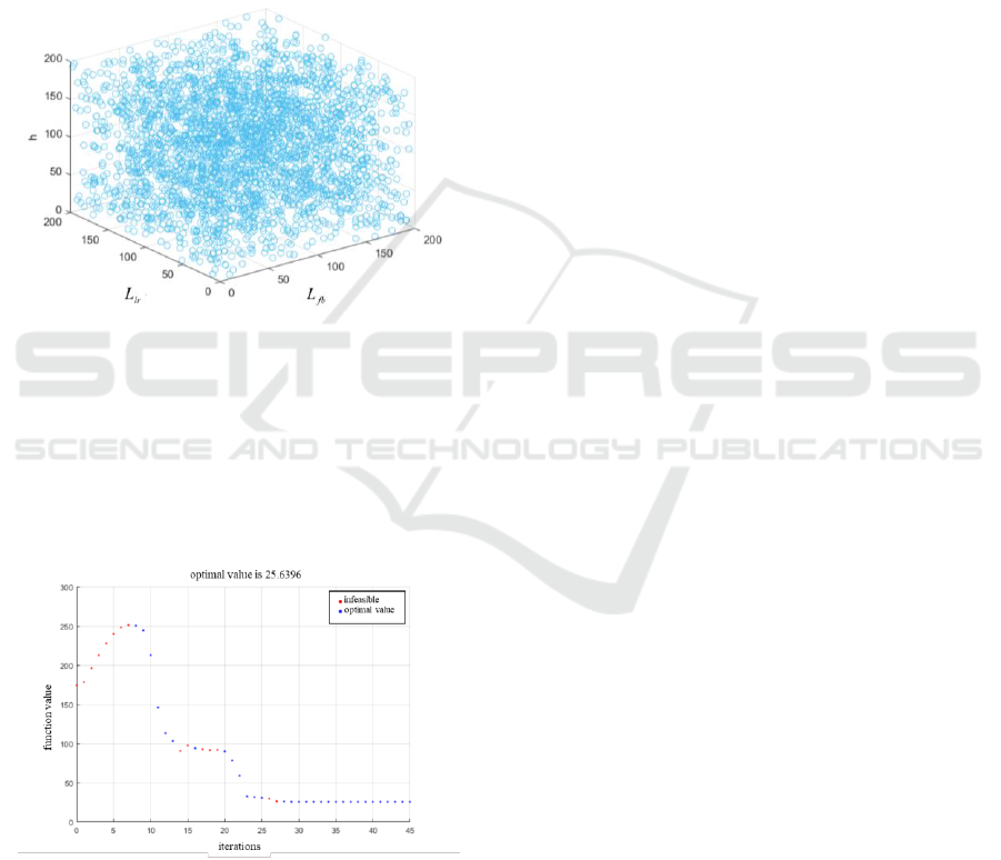
Figure 1: Initial value solution selection based on Monte
Carlo simulation.
Under the condition that
0.989
w
r
,
38.84
w
L
,
3
130Ge
,
88.8v
, temperature is 18
0
C
and air
pressure is 1014 hpa. The optimization model is
solved by MATLAB, shown in figure2.
Figure 2: Optimization procedure.
The optimal function value obtained is 25.6396,
and the optimal solution is
8.459 0.51310.5666
T
X , ,
.
The time difference between the front and back
engines is 17.1458s, which is in good agreement
with the actual situation.
ACKNOWLEDGMENTS
This work was financially supported by Dalian
Naval Academy research and innovation team fund
DJYKYKT2021-018 , and student research fund
DJYKYKT2022-003.
REFERENCES
Kamran Raissi, Mahmoud Mani, Mehdi Sabzehparvar,
Hooyar Ghaffari. A single heavy load airdrop and its
effect on a reversible flight control system [J]. Aircraft
Engineering and Aerospace Technology, 2008, 80(4):
1-9.
Wei T, Qu X, Wang L. Hierarchical mission planning for
multiple vehicles airdrop operation [J]. Aircraft
Engineering & Aerospace Technology, 2011,
83(5):315-323.
Min Xiao. Variable Structure Control of a Catastrophic
Course in a High-Speed Underwater Vehicle Launched
out of the Water [J]. Advances in Mechanical
Engineering, 2019, 5.
Zexiang Zhang, Zining Chen, Yong Zhao. Analysis on
General Reloading airdrop Loading Platform [J]. China
Equipment Engineering, 2021(08): 169-170.
Tianlin Qiang, Mengyuan Zhu. How difficult is reloading
airdrop [N]. PLA Daily, 2021-04-09(009).
Ri Liu, Xiuxia Sun, Wenhan Dong, Dong Wang. Adaptive
sliding mode control of airdrop gain for Transport
aircraft at Llow altitude [J]. Control Theory and
Applications, 2016, 33(10): 1337-1344.
Wenxing Wang, Dongchao Luo, Xiaomin Zhang, Xiuxia
Sun. Research on sliding mode control method of
second order terminal for reloaded airdrop of transport
aircraft [J]. Computer Measurement and Control, 2016,
24(09): 107-109.
Ri Liu, Yongbo Liu, Ming Xu, Siwei Yao, Peng Zhu.
Adaptive function approximate sliding mode control of
reloaded airdrop process [J]. Flight Mechanics,
2019(5): 45-50.
Research on Reloading Airdrop Strategy Based on Multi-Objective Programming
555
