The Classification of Tea Leaf Diseases Using Sift Feature Extraction of
Learning Vector Quantization Method with Support Vector Machine
Mutia Ulfa
1,2
, Rahmad Syah
1,2
and Muhathir
1,2
1
Informatics Depatrment, Faculty of Engineering, Universitas Medan Area, Medan, Indonesia
2
Excellent Centre of Innovations and New Science, Universitas Medan Area, Medan, Indonesia
Keywords:
Tea Leaf Diseases, Sift Feature Extraction, LVQ, SVM, Classification.
Abstract:
Productivity is highly dependent on healthy leaves, which are the main components of the product. However,
plants are very susceptible to all kinds of disturbances. One of these disturbances is a pest that causes disease
on tea leaves; the pest is helopeltis. is a type of pest that attacks young leaf shoots by piercing the part to be
attacked, and then the puncture mark from the razor will show symptoms in the form of irregular spots. Based
on the uniqueness of the damage pattern on the tea leaves, this study tested the classification of the types of tea
leaf diseases by comparing two methods, namely support vector machine and learning vector quantization, and
utilizing SIFT feature extraction. The level of accuracy produced by each method is 98% using the Support
Vector Machine method with 99% precision, 98% recall, and 98% F1-Score, and 94% using the Learning
Vector Quantization method with 96% precision, 94% recall, and 96% F1-Score.
1 INTRODUCTION
Artificial Neural Network (ANN), i.e., the model used
in problem solving to make decisions based on the
training provided (Cervantes et al., 2020), The ANN
concept is visible in the ANN working model, specif-
ically in the layer results and node output. ANN was
created to solve problems such as learning process
classification and pattern recognition. Backpropaga-
tion (slow training time, fast execution time), Boltz-
man (slow training and execution time), learning vec-
tor quantization (fast training and execution time),
and Hopfield are all monitored methods in ANN (fast
training time and moderate execution time). Based on
this method, it is clear that it has significant advan-
tages over the Learning Vector Quantization (LVQ)
method (Chen et al., 2021).
Learning Vector Quantization (LVQ) is a classifi-
cation method that uses a supervised layer for train-
ing. This layer can classify input vectors that are pro-
vided automatically. Some of the input vectors have
close weight values, so these weights will connect the
input layer with the competitive layer, which is the
layer that produces classes that are connected to the
output layer via the activation function. The LVQ al-
gorithm has two stages of training and testing that will
be used as a training and testing process. The initial
weight of the input values X1 to Xn is sent to the out-
put layer, which represents all classes, to determine
the maximum epoch (MaxEpoch), learning rate pa-
rameter (), reduced learning rate (Dec), and minimum
error (Eps). During the training stage, the LVQ calcu-
lations are used to generate weight values that will be
saved and used during the testing phase. During the
testing phase, new input data is classified by calculat-
ing the value of each weight in the input and selecting
the shortest distance between the two stored weights.
The class in the input image will be represented by the
value with the smallest weight distance (Guo et al.,
2023).
SVM is a nonlinear mapping algorithm that trans-
forms the original training data to a higher dimension.
In this case, the new dimension will seek a hyperplane
to separate linearly, and data from the two classes can
always be separated by a hyperplane with a precise
nonlinear mapping to a higher dimension (Kasisel-
vanathan et al., 2020). SVM is used to solve binary
classification problems. The goal is to find the best
hyperplane, not only by separating the two class la-
bels from the training sample, but also by defining
this hyperplane so that it is as far away from the clos-
est members of the two classes as possible (Kour and
Arora, 2019). SVM commonly employs linear, radial
basic function (RBF), and polynomial kernel func-
tions. The kernel functions and parameters used in
SVM analysis have a significant impact on the accu-
10
Ulfa, M., Syah, R. and Muhathir, .
The Classification of Tea Leaf Diseases Using Sift Feature Extraction of Learning Vector Quantization Method with Support Vector Machine.
DOI: 10.5220/0012439900003848
Paper published under CC license (CC BY-NC-ND 4.0)
In Proceedings of the 3rd International Conference on Advanced Information Scientific Development (ICAISD 2023), pages 10-14
ISBN: 978-989-758-678-1
Proceedings Copyright © 2024 by SCITEPRESS – Science and Technology Publications, Lda.

racy that is produced. The kernel function is a func-
tion that maps data to a higher-dimensional space in
the hope of improving the data’s structure and mak-
ing it easier to separate. Even if the hyperplane is
optimally determined in non-separable case training
data, the classification obtained may not have high
generalizability. As a result, the problem is solved
by mapping the input space into a high dimensional
dot-product space known as the feature space. Radial
Basic Function kernels are one type of kernel that is
used (RBF).
The RBF kernel function equation is:
k(x, x) = exp −
∥
x − x
′
∥
d
2σ
2
(1)
where d is the kernel degree.
A step in the image processing called feature ex-
traction is used to detect local features (Mokhtar et al.,
2015). The scale−invariant feature transform is used
in this study (SIFT). The Sift algorithm is skilled at
feature selection based on the appearance of an ob-
ject at a specific point of interest that is not affected
by image scale or rotation (Muhathir et al., 2019).
The sift algorithm requires two steps: extracting the
object’s characteristics and calculating its descriptors
(detecting the characteristics that most likely repre-
sent the object) and placing the matching steps as the
method’s ultimate goal (Nasution and Syah, 2022).
2 RESEARCH METHODOLOGY
Data collection method. Researchers collect data by
collecting sample data in the form of jpg images. The
images collected are based on the two classes that will
be classified: healthy leaves and leaves attacked by
the helopeltis pest. The total amount of data used in
this study was 1148, which was divided into 533 im-
ages of healthy leaf data and 615 images of helopeltis
pest-attacked leaves. Image captured with the Sam-
sung Galaxy A10 Smartphone at 13MP resolution.
The distance between data collection points is less
than 15 cm, and the background is white paper.
2.1 Data Analysis
Table 1 lists the 1148 images of healthy and helopeltis
diseased leaves that were used in this study. Table 2
shows how the 1148 data will be divided into training
and testing during the training and testing process.
Figure 2 depicts a research architecture that de-
picts the stages of research that will be carried out
Figure 1: Healthy Heaves.
Figure 2: Helopeltis Diseased
Leaves.
Table 1: Leaf data sharing.
Class Data Amount of Data
Healthy Leaves 533
Helopeltis Leaf Disease 615
Total 1148
Figure 3: Research Architecture.
using two processes: training and testing. The train-
ing procedure begins with the entry of image data
in the form of images from research results on tea
leaf images, followed by grayscale conversion using
SIFT feature extraction and weight storage (Prabu and
Chelliah, 2023). Importing image data in the form of
images derived from tea leaf image research, convert-
ing the images to grayscale using SIFT feature extrac-
tion, and storing the weights. Extraction of grayscale
image data from three color spaces, R, G, and B, into
one color space, grayscale, and then extraction using
SIFT feature extraction results in the data being stored
as a pattern model that will be used in the testing
process (Saputra, 2020). The second testing proce-
dure involves training matching pattern models using
the Learning Vector Quantization and Support Vector
Machine classification methods.
The Classification of Tea Leaf Diseases Using Sift Feature Extraction of Learning Vector Quantization Method with Support Vector Machine
11

Table 2: Distribution of training and testing data.
Overall Data Sharing Amount of Data
Training 80% 918
Testing 20% 230
2.2 Pre-Processing Data
The leaf image will now be measured by shrinking the
pixel size. When I started, the tea leaf image was still
4128 x 3096 pixels. The data will then be cropped to
emphasize the main object in the image. The image
size is increased to 300 x 400 pixels after cropping to
make it more effective for tea leaf image processing.
The 1148 tea leaves used in this study were divided
into two groups: healthy leaves (533 total images) and
helopeltis disease leaves (533 total images) (615 im-
ages total).
3 RESULTS AND DISCUSSION
Data is illustrated as an array. The data that is input
and then read by the machine into an array is depicted
below.
Figure 4: Illustration of Data.
1. SIFT Feature Extraction Step 1:
F(a, b, σ) =
(G(a, b, , kσ)) ∗ 1(a, b)
= L(a, b, kσ)−
L(a, b, σ)
(2)
Step 2: Get the keypoint
Step 3:
s(a, b) =
p
(L(a + 1, b) − L(a − 1, b))2+
p
(L(a, b + 1) − L(a, b − 1))2
(3)
θ(a, b) =
tan
−1
(
L(a, b − 1) − L(a, b − 1
L(a + 1, b) − La − 1, b
)
(4)
The following is the result of the tea leaf image
using feature extraction using SIFT (Scale Invari-
ant Feature Transform). Can be seen in Figures 5
and 6.
Figure 5: Pictures of Helopeltis Leaves.
Figure 6: Pictures of SIFT Extraction Results.
2. Confusion Matrix The following is the result of
the confusion matrix from the Learning Vector
Quantization and Support Vector Machine meth-
ods. Can be seen in Figures 7 and 8.
Figure 7: Results of the confusion matrix from the Learning
Vector Quantization Method.
3. Evaluation Model
a. Learning Vector Quantization LVQ denotes a
collection of vector prototypes of S, one or
more of which can be assigned to each class. In
the feature space, prototype vectors are identi-
fied and serve as typical representatives of each
class.
a =
{
a
i
, b(a
i
}
s
i=1
b(a
i
)ε
{
1, 2, 3, ..., X
}
(5)
Along with a certain distance d(c, a), the
ICAISD 2023 - International Conference on Advanced Information Scientific Development
12

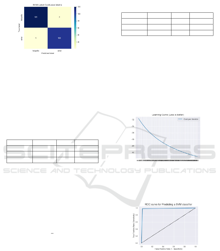
Figure 8: Results of the confusion matrix from the Support
Vector Machine Method.
values make up the classification scheme pa-
rameters. The Winner schema takes all values,
i.e.: arbitrary input X is assigned to class j(a
L
)
of the closest prototype to d(c, a
L
) ≤ d(c, a
i
)
for all i.
The following is a performance evaluation of
image classification on tea leaves extracted
with the SIFT feature using the LVQ method:
Table 3: Evaluation of Tea Leaf Image Classification Per-
formance Using the LVQ Method.
Precision Recall F1-Score
Helopeltis 0.96 0.94 0.96
Healthy 0.94 0.95 0.94
Accuracy 0.94
The results of the research evaluation model
using the LVQ algorithm are shown in Ta-
ble 3. The precision, recall, and F1-score of
Helopeltis leaves are all 96%. While healthy
leaves have a precision of 94%, a recall of
95%, and an F1-score of 94%, LVQ results in
an accuracy of 94% (Wady et al., 2020).
b. Support Vector Machine Kernel function used
in svm
minα
1
2
α
T
Cα − e
T
α
a.t.0 ≤ X , i = 1, ..., l
b
T
α = 0
(6)
The following is an evaluation of performance
in image classification on tea leaves that have
been extracted with the SIFT feature with
SVM:
The results of the research evaluation model
using the SVM algorithm are shown in Table
4. Helopeltis leaves have 99% precision, 98%
recall, and an F1-score of 98%. While healthy
leaves have a precision of 97%, a recall of
Table 4: Evaluation of Tea Leaf Image Classification Per-
formance Using the SVM Method.
Precision Recall F1-Score
Helopeltis 0.99 0.98 0.98
Healthy 0.97 0.99 0.98
Accuracy 0.98
99%, and an F1-score of 98%, SVM results in
an accuracy of 98% (Wang et al., 2019).
4. Curve Method The ROC (Receiver Operating
Characteristic) curve is used to show the results of
the research. The ROC curve is made based on the
value obtained in the calculation with the confu-
sion matrix, namely between False Positive Rate
and True Positive Rate vector prototypes of S, of
which one or more prototypes can be assigned to
each class. In the feature space, prototype vectors
are identified and serve as typical representatives
of each class.
Figure 9: Image of LVQ Iteration Curve.
A representation of the LVQ learning curve,
specifically the performance of the generated
LVQ algorithm. The resulting curve decreases, in-
dicating that the LVQ performance is satisfactory.
Figure 10: ROC Curve Svm Image.
The image above depicts the ROC (Receiver Op-
erating Characteristic) curve obtained from SVM
classification.
From the ROC curve in figure 9, the results are
obtained: ROC AUC : 0.9831 Cross Validate ROC
AUC : 0.9986.
The Classification of Tea Leaf Diseases Using Sift Feature Extraction of Learning Vector Quantization Method with Support Vector Machine
13

4 CONCLUSION
This study compares two methods for classifying tea
leaf disease, namely Support Vector Machine and
Learning Vector Quantization, and employs SIFT fea-
ture extraction. Each method achieves 98% precision,
98% recall, and 98% F1-score, while Learning Vector
Quantization achieves 96% precision, 94% recall, and
96% F1-score.
REFERENCES
Cervantes, J., Garcia-Lamont, F., Rodr
´
ıguez-Mazahua,
L., and Lopez, A. (2020). A comprehensive sur-
vey on support vector machine classification: Ap-
plications, challenges and trends. Neurocomputing,
408:189–215.
Chen, S., Zhong, S., Xue, B., Li, X., Zhao, L., and
Chang, C.-I. (2021). Iterative scale-invariant fea-
ture transform for remote sensing image registration.
IEEE Transactions on Geoscience and Remote Sens-
ing, 59(4):3244–3265.
Guo, J., Wang, Z., and Zhang, S. (2023). Fessd: Feature
enhancement single shot multibox detector algorithm
for remote sensing image target detection. Electron-
ics, 12(4):946.
Kasiselvanathan, M., Sangeetha, V., and Kalaiselvi, A.
(2020). Palm pattern recognition using scale invari-
ant feature transform. International Journal of Intelli-
gence and Sustainable Computing, 1(1):44.
Kour, V. and Arora, S. (2019). Particle swarm optimiza-
tion based support vector machine (p-svm) for the seg-
mentation and classification of plants. IEEE Access,
7:29374–29385.
Mokhtar, U., Ali, M., Hassanien, A., and Hefny, H. (2015).
Identifying two of tomatoes leaf viruses using support
vector machine.
Muhathir, R., A., R., Sihotang, J., and Gultom, R. (2019).
Comparison of surf and hog extraction in classifying
the blood image of malaria parasites using svm. In
2019 International Conference of Computer Science
and Information Technology (ICoSNIKOM, page 1–6.
Nasution, M. and Syah, R. (2022). Data management as
emerging problems of data science. In Data Science
with Semantic Technologies, page 91–104. Wiley.
Prabu, M. and Chelliah, B. (2023). An intelligent ap-
proach using boosted support vector machine based
arithmetic optimization algorithm for accurate detec-
tion of plant leaf disease. Pattern Analysis and Appli-
cations, 26(1):367–379.
Saputra, A. (2020). Penentuan parameter learning rate se-
lama pembelajaran jaringan syaraf tiruan backprop-
agation menggunakan algoritma genetika. Jurnal
Teknologi Informasi: Jurnal Keilmuan dan Aplikasi
Bidang Teknik Informatika, 14(2):202–212.
Wady, S., Yousif, R., and Hasan, H. (2020). A novel in-
telligent system for brain tumor diagnosis based on a
composite neutrosophic-slantlet transform domain for
statistical texture feature extraction. BioMed Research
International, page 1–21.
Wang, Y., Zhu, X., and Wu, B. (2019). Automatic detection
of individual oil palm trees from uav images using hog
features and an svm classifier. International Journal
of Remote Sensing, 40(19):7356–7370.
ICAISD 2023 - International Conference on Advanced Information Scientific Development
14