
HBP: A NOVEL TECHNIQUE FOR DYNAMIC OPTIMIZATION
OF THE FEED-FORWARD NEURAL NETWORK
CONFIGURATION
Allan K.Y. Wong , Wilfred W.K. Lin
Department of Computing, Hong Kong Polytechnic University, Hung Hom, Kowloon, Hong Kong SAR,
Tharam S. Dillon
Faculty of Information Technology, University of Technology, Sydney Broadway, N.S.W. 2000,
Keywords: Hessian-based pruning technique, Internet, Tay
lor series, dynamic, NNC
Abstract: The novel Hessian-based pruning (HBP) technique to optimize the feed-forward (FF) neural network (NN)
configuration in
a dynamic manner is proposed. It is then used to optimize the extant NNC (Neural Network
Controller) as the verification exercise. The NNC is designed for dynamic buffer tuning to eliminate buffer
overflow at the user/server level. The HBP optimization process is also dynamic and operates as a renewal
process within the service life expectancy of the target FF neural network. Every optimization renewal cycle
works with the original NN configuration. In the cycle all the insignificant NN connections are marked and
then skipped in the subsequent operation before the next optimization cycle starts. The marking and
skipping operations together characterize the dynamic virtual pruning nature of the HBP. The interim
optimized NN configuration produced by every HBP cycle is different, as the response to the current system
dynamics. The verification results with the NNC indicate that the HBP technique is indeed effective because
all the interim optimized/pruned NNC versions incessantly and consistently yield the same convergence
precision to the original NNC predecessor, and with a shorter control cycle time.
1 INTRODUCTION
The novel Hessian-based pruning (HBP) technique
proposed in this paper is for dynamic optimization
of feed-forward neural network configurations. It
operates as a renewal process within the life
expectancy of the target neural network. In every
renewal cycle all the weights of the arcs in the
original NN configuration are re-computed. Then,
the significance of the arcs/connections is sorted by
the impact of the weight on the NN convergence
accuracy. Those insignificant arcs are first identified
and then skipped in the NN operation between two
successive optimization cycles. The suite of
activities: cyclic computation of arc weights,
marking them, and skipping them is known as
dynamic optimization (virtual pruning) in the HBP
context. The HBP technique is verified with the
NNC (Neural Network Controller) (Lin, 2003) with
a FF configuration. The aim of the NNC is to
provide dynamic buffer tuning (Ip, 2001, Wong,
2002) that eliminates buffer overflow at the
user/server level. The preliminary experimental data
indicates that the interim optimized NNC (ONNC)
versions never fail to perform with the same
precision as the un-optimized NNC predecessor (Lin,
2002) with a shorter control cycle time.
2 RELATED WORK
Using controllers to smoothen out industrial
processes has a long and successful history. The
traditional controllers usually combine the P
(proportional), D (derivative) and I (integral) control
elements in different ways. For example, the PID (i.e.
“P+I+D”) controller is the most widely used in
industry. The modern controllers involve soft
computing techniques, such neural network, genetic
algorithms, and fuzzy logic extensively. Therefore,
industrial controllers can be hard-algorithmic models
that base on mathematical models or
346
K. Y. Wong A., W.K. Lin W. and S. Dillon T. (2004).
HBP: A NOVEL TECHNIQUE FOR DYNAMIC OPTIMIZATION OF THE FEED-FORWARD NEURAL NETWORK CONFIGURATION.
In Proceedings of the First International Conference on Informatics in Control, Automation and Robotics, pages 346-349
DOI: 10.5220/0001126103460349
Copyright
c
SciTePress

expert/intelligent mechanisms that adapt the control
parameters dynamically at runtime. Recently the
control techniques for industrial processes are being
transferred and adapted for dynamic buffer tuning.
The objective is to prevent buffer overflow in
Internet TCP channels (Braden, 1998). The NNC is
one of the expert controller models designed to
eliminate buffer overflow at the user-level (Lin,
2002, Wong, 2002). But, it has two distinctive
shortcomings:
a) It has a long control cycle time that would lead to
deleterious effect, which means that by the time
the corrective action is computed the actual
problem to be rectified has already gone.
b) It is difficult to decide when the NNC controller
is sufficiently trained on-line.
The NNC is a FF neural network that works by
backpropagation and controls with the
objective function. It consistently maintains the
given
safety margin about the reference
QOB
ratio or
QOB
(represented by the “0” in ).
2
},0{ ∆
∆
R
The problem of the NNC real-life application is its
long average control cycle time (CTC) of 10800
clock/T cycles. The CTC is measured with the
Intel’s VTune Performance Analyzer (Vtune). The
neutral clock cycles can be converted into the
physical time for any platform of interest. For
example, if the NNC is running on a platform
operating at
MHz, then the physical CTC
T
2
},0{ ∆
800=f
physical
is:
ockCycle
s
NumberOfCl
f
T
physical
*
1
=
implying
. The previous analysis (Lin,
2002) indicates that the long CTC diminishes the
chance of deploying the NNC for serious real-time
applications, especially over the Internet. The
control accuracy of the NNC, however, makes it
worthwhile to optimize its configuration in a
dynamic manner so that the
in operation is
consistently reduced. For this reason the NNC is
chosen as the test-bed for the novel HBP technique.
The “HBP+NNC” combination is known as the
Optimized NNC (ONNC) model.
ms0135.0
physical
T
3 THE HESSIAN-BASED
PRUNING TECHNIQUE
The HBP operation is based on dynamic sensitivity
analysis. The rationale is to mark and inhibit/skip a
FF neural network connection if the error/tolerance
of the neural computation is insensitive to its
presence. For the NNC the error/tolerance is the
ed by “0” in th
2
}∆ objective function.
The core argument for t technique is: “if a
neural network converges toward a target function
so will its derivatives (Gallant, 1992)”. In fact, the
main difference among all the performance-learning
laws identified from the literature (Hagan, 1996) is
how they leverage the different parameters (e.g.
weights and biases). The HBP adopts the Taylor
Series (equation (3.1)) as the vehicle to differentiate
the relative importance of the different neural
network (NN) parameters. The meanings of the
parameters in equation (3.1) are: F() - the function,
w - the NN connection weight,
∆
w – the change in w,
∇
F(w) - the gradient matrix, and ∇
∆± band about th reference, symbolically
mark
,0{
he HBP
e
R
QOB
e
2
F(w) - the
Hessian matrix. The other symbols in the equations
are: T for transpose, O for higher order term, n for
the n
th
term, and
1
w∂
∂
for partial differentiation.
F(w+
∆
w) = F(w) +
∇
F(w)
T
∆
w
+
2
1
∆
w
T
∇
2
F(w)
∆
w + O(||
∆
w ||
3
)+……(3.1)
F(w): ∇
)2.3(..........
21
)()...()(
⎥
⎦
⎤
⎢
⎣
⎡
∂
∂
∂
∂
∂
∂
wF
w
wF
w
wF
w
n
T
∇
2
F(w):
)3.3.........(
)(...)()(
............
)(...)()(
)(...)()(
2
1
2
⎢
⎢
⎡
∂
∂
wF
2
2
2
2
1
2
2
2
2
2
2
12
2
1
2
21
2
⎥
⎥
⎥
⎥
⎥
⎥
⎥
⎥
⎥
⎥
⎦
⎤
⎢
⎢
⎢
⎢
⎢
⎢
⎢
⎢
⎣
∂
∂∂∂∂
∂∂
∂
∂∂
∂∂∂
∂∂∂
∂∂∂
∂∂
wFwFwF
wFwFwF
wFwF
w
wwww
ww
w
ww
wwww
w
n
nn
n
n
The preliminary ONNC verification results confirm
that the HBP performs as expected and concur with
the previous experience. With the equation (3.1) the
learning/training process should converge to the
R
QOB
reference, which is mathematically called
the get global minimum surface. The convergence
makes the gradient vector
∇
F(w) insignificant and
eliminates the “
∇
F(w)
tar
T
∆
w” term from equation
(3.1). This implies not only that the larger ordinal
terms in equation (3.1) can be ignored but also a
possible simpler form (equation (3.4)). Further
simplification of equation (3.4) based on:
∆
F=F(w+
∆
w)-F(w), yields equation (3.5).
F(w+∆w) = F(w) +
2
1
∆w
T
∇
2
F(w)∆w…(3.4)
∆F=
2
1
∆w
T
∇
2
F(w)∆w…(3.5)
H ss is applied to the
Learner immediately after it has completed training
The BP optimization proce
HBP: A NOVEL TECHNIQUE FOR DYNAMIC OPTIMIZATION OF THE FEED-FORWARD NEURAL NETWORK
CONFIGURATION
347
and before it swaps to be the Chief. The details
involved are as follows:
Use Taylor series (equation (3.1)) to identify the
significant neural network parameters.
tions.
its neural computation.
ctions is
Choose appropriate learning rates for the significant
parameters to avoid convergence oscilla
Mark the synaptic weights that have insignificant
impact on the Taylor series.
After the Learner has become the Chief, it excludes
all the marked connections in
The exclusion is represented by equation (3.6), and
the net effect is the virtual pruning of the
insignificant connections. In every optimization
cycle within the service life of the target neural
network the same skeletal FF configuration is
always the basis for pruning, based on the
Lagrangian index S (to be explained later).
In the initial phase of the optimization cycle the
importance of all the neural network conne
sorted by their weights. For example, for the NNC
these weights represent the different degrees of
impact on the convergence speed and accuracy. The
fact that the HBP optimization is a renewal process
makes it dynamic and adaptive.
w
i
+
∆
wi
=0…(3.6)
)()(
2
w
wFS ∆=
∇
y equatio
1
2
wU
TT
ww +∆−∆
λ
ii
…(3.7a)
If
∆
w in equation (3.5) is replaced b n (3.6),
then the Lagrangian equation (3.7a) is formed. Now
equation (3.1) is a typical constrained optimization
problem. The symbols:
U
T
i
and λ in equation (3.7b)
are the unit vector and the Lagrange multiplier
respectively. The optim change in the weight
vector w
um
i
(equation (3.6)) is shown in equation
(3.7b). Every entry in w
i
associates with a unique
Lagrangian index S
i
(equation (3.7c)). In the HBP
optimization cycle the S
i
values are sorted so that the
less significant w
i
(connection weight) is excluded
from the operation. For the NNC twin system the
exclusion/pruning starts from the lowest S
i
for the
Learner and stops if the current exclusion affects the
convergence process. Only after the pruning process
has stopped that the Learner can become the Chief.
U
wF
wF
w
i
ii
i
wi
)(
])([
2
1
2
1
,
∇
∇
−
−
−=∆
…(3.7b)
..
1
2
2
]
)(
[
,
2
wF
w
S
ii
i
i
−
=
∇
4 THE PRELIMINARY ONNC
RESULTS
Different ONNC optimization experiments were
conducted. The preliminary verification results indicate
that the HBP technique is indeed effective for pruning of
the NNC configuration in the cyclical and dynamic
manner. The skeletal configuration for the ONNC
prototype is 10 input neurons, 20 neurons for the hidden
layer, and one output neuron. This FF neural network
configuration is fully connected, with 200 connections
between the input layer and the hidden layer, and 20
connections between the hidden layer and the output layer.
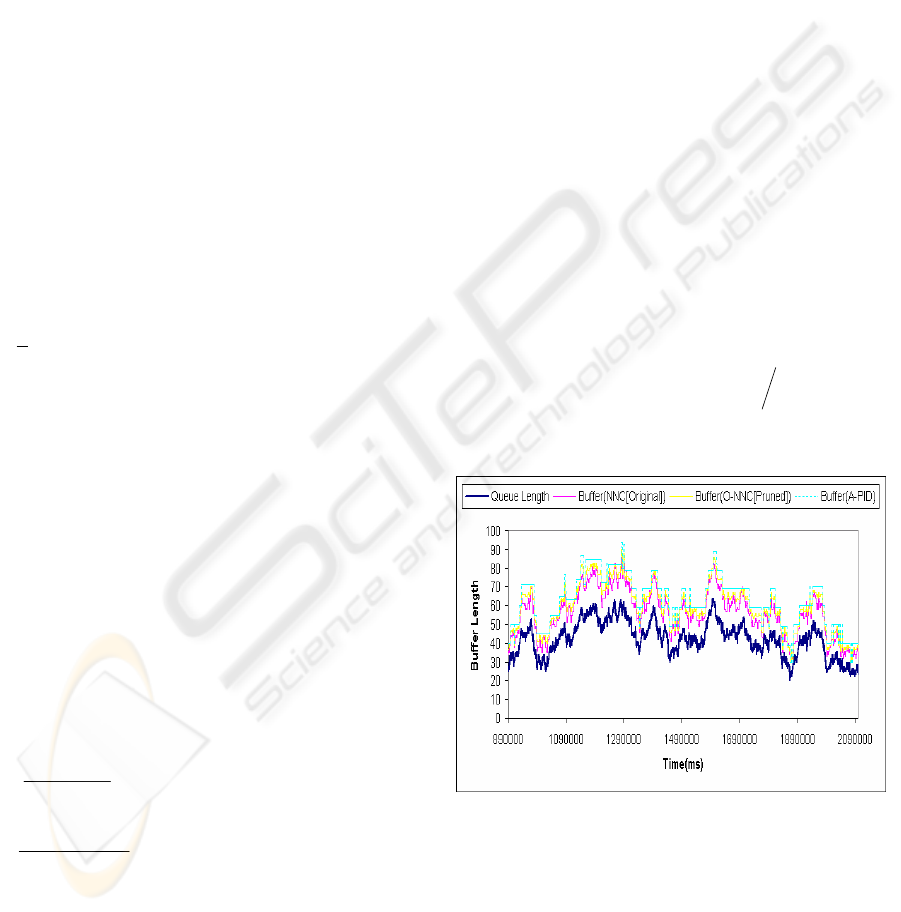
Figure 1 compares the control output of the NNC, the
ONNC and the algorithmic PID controller (Lin, 2002).
The PID controller always prevents buffer overflow at the
server level, and it is used here for comparative purpose
with the same input data. The hidden layer in the ONNC
has only 187 connections on average after the HBP
optimization, instead of the original 220 in the skeletal
configuration. That is, 33 of connections are
skipped/pruned under the HBP control. The most
important of all is that the experimental results in the
verification exercise confirm that the interim ONNC
versions always produce the same level of buffer overflow
elimination efficacy as the un-optimized NNC, with
shorter control cycle times. The ONNC, however, has a
larger mean deviation (MD) than the un-optimized NNC,
with MD defined as:
kQOBMD
k
i
i
⎥
⎦
⎤
⎢
⎣
⎡
−∆=
∑
=1
||
. The average
ONNC control cycle time is only 9250 clock pulses
compared to the 10800 for the up-optimized predecessor.
Figure 1: A NNC optimization/pruning experimental result
…(3.7c)
For comparative purposes, Table 1 summarizes the
average amount of buffer size adjustment (in ratio)
for two actual cases: “Case 1” and “Case 2” by four
different controllers designed for dynamic buffer
tuning. The input traffic to these controllers are the
same, and the adjustment size in ratio is calculated
with respect to the current buffer size, which is taken
as 1 or 100%. For example, the mean PID
ICINCO 2004 - INTELLIGENT CONTROL SYSTEMS AND OPTIMIZATION
348

adjustment change/size in “Case 1” is 0.14 or 14%
for either the buffer elongation or the shrinkage
operation. That is, the average amplitude of dynamic
buffer tuning for “Case 1” is 0.28 or 28%. The
traffic pattern of the TCP channel during the “Case
1” experiment is heavy-tailed, as confirmed by the
Selfis Tool (Karagiannis, 2003). The pattern for
“Case 2” is random because the mean m of the
distribution for the traffic trace is approximately
equal to its standard deviation
δ
(i.e.
δ
≈m
).
Table 1: A summary of the average buffer adjustment size
and amplitude
PID (Ip,
2001) ONNC
FLC
(Lin, 2003)
GAC
(Wong,
2002)
Traffic
pattern
Case 1 – mean
adjustment size
0.140 0.0265 0.0267 0.0299
Heavy-
tailed
(i.e.
LRD)
(mean adjustment
amplitude)
≈ ≈0.28
4
0.05
3
≈ 0.053 ≈ 0.06
Case 2 – mean
adjustment size
0.1373 0.0293 0.0296 0.0324
Random
Mean adjustment
size (in ratio) for
20 different study
cases
0.139 0.0279 0.0282 0.0311
Mean adjustment
amplitude (in ratio)
for above 20
different cases
≈ 0.27
7
≈ 0.05
6
≈ 0.056
≈ 0.06
2
5 CONCLUSION
The HBP technique is proposed for dynamic cyclical
optimization of FF neural network configurations
(e.g. the NNC). The optimization is, in effect, virtual
pruning of the insignificant NN connections. With
the NNC every HBP optimization cycle starts with
the same skeletal configuration. The experimental
results show that the interim ONNC versions always
have a shorter control cycle time. The ONNC model
is actually the “HBP+NNC” combination. The
verification results indicate that the average ONNC
control cycle time is 14.3 percent less than that of
the un-optimized NNC predecessor. In the
optimization process the connections of the NNC are
evaluated and those have insignificant impact on the
dynamic buffer tuning process are marked and
virtually pruned. The pruning process is logical or
virtual because it does not physically remove the
connections but excludes them in the neural
computation only. The HBP is applied solely to the
stage when Learner has just completed training and
before it swaps to assume the role as the Chief.
ACKNOWLEDGEMENT
The authors thank the Hong Kong PolyU for the
research grants: A-PF75 and G-T426.
REFERENCES
B. Braden et al., Recommendation on Queue Management
and Congestion Avoidance in the Internet, RFC2309,
April 1998
Allan K.Y. Wong, Wilfred W.K. Lin, May T.W. Ip, and
Tharam S. Dillon, Genetic Algorithm and PID Control
Together for Dynamic Anticipative Marginal Buffer
Management: An Effective Approach to Enhance
Dependability and Performance for Distributed Mobile
Object-Based Real-time Computing over the Internet,
Journal of Parallel and Distributed Computing (JPDC),
vol. 62, Sept. 2002
A. R. Gallant and H. White, On Learning the Derivatives
of an Unknown Mapping and Its Derivatives Using
Multiplayer Feedforward Networks, Neural Networks,
vol. 5, 1992
M. Hagan et al, Neural Network Design, PWS Publishing
Company, 1996
T. Karagiannis, M. Faloutsos, M. Molle, A User-friendly
Self-similarity Analysis Tool, ACM SIGCOMM
Computer Communication Review, 33(3), July 2003,
81-93
Wilfred W.K. Lin, An Adaptive IEPM (Internet End-to-
End Performance Measurement) Based Approach to
Enhance Fault Tolerance and Performance in Object
Based Distributed Computing over a Sizeable
Network (Exemplified by the Internet), MPhil Thesis,
Department of Computing, Hong Kong PolyU, 2002
Wilfred W.K. Lin, Allan K.Y. Wong and Tharam S.
Dillon, HBM: A Suitable Neural Network Pruning
Technique to Optimize the Execution Time of the
Novel Neural Network Controller (NNC) that
Eliminates Buffer Overflow, Proc. of Parallel and
Distributed Processing Techniques and Applications
(PDPTA), vol. 2, Las Vegas USA, June 2003
May T.W. Ip, Wilfred W.K. Lin, Allan K.Y. Wong,
Tharam S. Dillon and Dian Hui Wang, An Adaptive
Buffer Management Algorithm for Enhancing
Dependability and Performance in Mobile-Object-
Based Real-time Computing, Proc. of the IEEE
ISORC'2001, Magdenburg, Germany, May 2001
IIntelVtune,
http://developer.intel.com/software/products/vtune/
HBP: A NOVEL TECHNIQUE FOR DYNAMIC OPTIMIZATION OF THE FEED-FORWARD NEURAL NETWORK
CONFIGURATION
349
