
AN INSTRUMENT CONTROL SYSTEM USING PREDICTIVE
MODELLING
Geoffrey Holmes and Dale Fletcher
University of Waikato, Department of Computer Science, Hamilton, New Zealand.
Keywords: Machine learning, control applications
Abstract: We describe a system for providing early warning of possible error to an operator in control of an
instrument providing results in batches from samples, for example, chemical elements found in soil or water
samples. The system has the potential to be used with any form of instrument that provides multiple results
for a given sample. The idea is to train models for each measurement, using historical data. The set of
trained models are then capable of making predictions on new data based on the values of the other
measurements. This approach has the potential to uncover previously unknown relationships between the
measurements. An example application has been constructed that highlights the difference of the actual
value for a measurement from its predicted value. The operator is provided with sliders to attenuate the
sensitivity of the measurement perhaps based on its importance or its known sensitivity.
1 INTRODUCTION
Machine learning is the driving force behind data-
driven modelling. This is in contrast to modelling an
application using a physical model (mathematical or
probabilistic) which is prescribed a priori and then
tested against actual data. This process is also
referred to as predictive modelling. Data-driven
modelling involves a number of steps following the
collection of data. These steps may involve the
removal of outliers, noise reduction, data
transformation and so on. Collectively they represent
a cleansing process which prepares the data for an
induction step where models are learnt directly from
the data.
In the physical modelling scenario domain
kn
owledge can be added directly to the model. For
most machine learning techniques (except for
example those based on inductive logic
programming) such knowledge can only be
introduced at the cleansing stage.
Once a model has been induced it is tested
agai
nst new data and evaluated on some
performance criteria. If the model is transparent then
it can be examined as a reality check. This process
can, in fact, provide unexpected insights into the
data. Generally the process is iterative as insights or
poor performance can lead to changes in the earlier
processing steps.
By far the most common use of machine learning
in
control applications is in the field of robotics.
This is in part due to the close relationship between
the two subject areas but also reflects the ease with
which such applied projects can be carried out.
Commercial control applications in the literature are
somewhat rarer although there have been a number
of successes.
Any process control application involving the
settin
g of a complex array of mutually dependent
parameters is a target for machine learning.
Examples include controlling printing presses
(Evans and Fisher, 2002), the manufacture of
nuclear fuel pellets (Langley and Simon, 1995), and
the separation of oil and natural gas (Slocombe et al,
1986). In general, the technology is suited to
applications involving a large, possibly infinite,
source of stable data, that is, a source which does not
undergo major changes in format. It is also suited to
applications which preclude physical modelling due
to their inherent complexity. In such circumstances
it is possible to also consider hybrids, combinations
of physical and data-driven models.
This paper is organised as follows. Section 2
p
rovides a context in which the predictive modelling
is taking place. Section 3 describes the modelling
technique used in this paper. Section 4 gives an
overview of the architecture of the entire system,
which is web-based. We conclude in Section 5 with
292
Holmes G. and Fletcher D. (2004).
AN INSTRUMENT CONTROL SYSTEM USING PREDICTIVE MODELLING.
In Proceedings of the First International Conference on Informatics in Control, Automation and Robotics, pages 292-295
DOI: 10.5220/0001126602920295
Copyright
c
SciTePress
observations and ideas for future system
development.
2 EXPERIMENTAL DESIGN
In this paper we refer to the following experimental
setup. We suppose the existence of an instrument
capable of simultaneously measuring a number of
properties of some substance presented as a sample.
In machine learning, these measurements are
typically referred to as attributes of the sample.
Suppose further that the instrument is extremely
efficient in processing a sample and so the setup
enables the concatenation of samples into batches.
For a given sample of n measurements we seek a
model (for example, a linear regression) for each
measurement based on the remaining n-1
measurements.
The system is constructed in two phases. A
training phase where historical data is used to train
models for each measurement, and a prediction
phase where the measurement values for new
samples (not part of the training data) are predicted
using the trained models. This methodology is built
on the assumption that measurements are generally
stable when taken as a simultaneous group and that
the various measurements are therefore reliable
predictors of each other. Instability in particular
measurements will show up as a variance between
the actual value of the measurement and the
predicted value. If it is possible to view the trained
models then a further advantage of this approach is
that it may be possible to discover (in a data mining
sense) previously unknown correlations between
measurements. For example, one measurement may
be a perfect predictor for another and this
relationship may not have been known a priori.
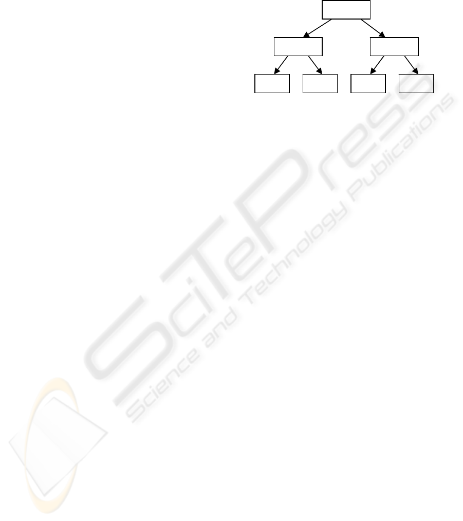
3 MODEL TREES
As most instruments produce measurements as
floating point values some form of regression is
needed to produce models. The WEKA data mining
workbench (Witten and Frank, 2000) contains a
number of candidate regression methods. After
experimenting with several of these techniques we
decided to use model trees (Wang and Witten,
1997). The interior nodes of a model tree contain
tests that split the data on a particular value for a
The leaves of a model tree contain linear regression
functions modelling those examples that fall to the
leaf following the execution of the various tests in
the interior nodes of the tree. A typical model tree is
shown in Figure 1.
particular measurement. The algorithm attempts to
choose tests that “best” split the data into groups. A
test’s height in the tree is an indicator of how
important that measurement is in splitting the data.
ediction
ge number of measurements, which has
eful measurements
we used some of WEKA’s filtering capability to
remove irrelevant measurements, that is, those that
s of the
alert an operator
of potential measurement errors. Second, a
visualisation component to allow an operator to
interactively adjust the thresholds (which may have
an effect on the first component).
Figure 1: Sample model tree
We label the measurements m1, m2, and so on. The
model tree algorithm attempts to divide the training
data into groups and attaches to each group the
linear model that best fits that group of data (using
linear regression). The branches labelled t (for true)
are followed if the test is satisfied, otherwise the f
(for false) branch will be followed. Thus, the LM1
linear model will only apply to data points with m1
values less than 10 and m2 values greater than 5.
Once trained, this model can be used for pr
purposes as each untrained data sample will fall to
one of the linear models in the tree and receive a
prediction value from that model. Recall that a
model is constructed for each measurement.
In any practical system, the instrument may
produce a lar
implications for the system overall. Only a limited
amount of memory is available for modelling so not
necessarily all measurements can be or indeed need
be covered.
In order to find the set of us
do not appear in either the interior node
model trees or in the leaf nodes.
4 SYSTEM DESCRIPTION
The models described in Section 3 are only a part of
the overall system. The complete architecture is
shown in Figure 2. The system, which has been
designed to function as a web service, has two main
components. First, a component to
m1 < 10
m2 > 5 m4 < 2.6
LM1 LM2 LM4LM3
t
t
f
f
f
t
AN INSTRUMENT CONTROL SYSTEM USING PREDICTIVE MODELLING
293
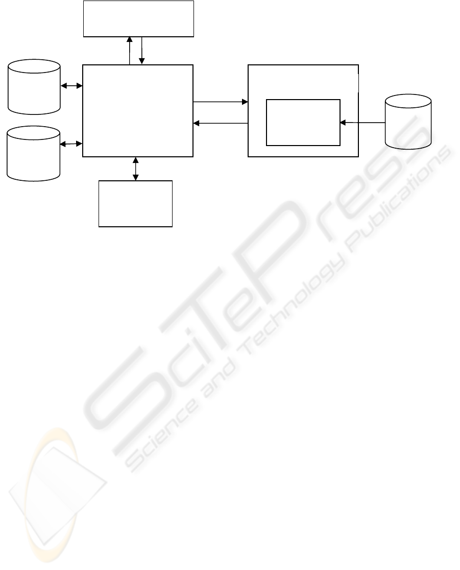
A measurement comprises two components, an
identifier describing the measurement and a numeric
value. A completed batch of measurements is placed
into an XML stream and sent by the instrument
(more typically an instrumentation system) to a web
service on the web application server. The role of
the web application server is to manage
communication with the WEKA Prediction Engine
through the Java application server, and to return an
appropriate response back to the instrument for an
operator to action.
The measurements are re-packaged (the data
formats of the instrument and machine learning
components need to be aligned) and passed to the
WEKA Prediction Engine, which has pre-loaded
serialised models for each measurement from the
models database.
Because the instrument may be programmed to
produce only a subset of measurements, and new
measurements may come online at any time, it is
important that the system is designed to be able to
process any number and combination of
measurements. The architecture supports possible
changes in the instrumentation system through its
XML interfaces and database of models.
For each set of measurements in a batch, a
WEKA Instance is created, with measurement
identifiers as attributes. At this stage it is ensured
that the WEKA Instance created only includes those
measurements used by the models. Any
measurement (attribute) used by the models but not
present in the measurement set, is added to the
Instance, and set to have a missing value.
Missing values can cause difficulties, as
classifiers do not always treat them appropriately.
Many classifiers, for example, replace missing
values with a mean value and this can be grossly
incorrect for some measurements. Recall that we are
trying to predict a single measurement from linear
combinations of other measurements. If within the
linear combination there is a highly weighted
measurement for which the Instance contains a
missing value, then we do not generate a prediction
for that Instance. The system is designed to alert the
operator to potentially abnormal measurements. The
use of means for missing values is too unstable a
predictor and leads to setting larger tolerances on
measurements which in turn leads to a greater
likelihood of ignoring real errors.
The WEKA Prediction Engine produces
predicted values for each measurement, using
models previously trained on a large history of
measurements. For each individual measurement in
the set, the models database is searched to find a
model with matching identifier. If one is found, the
model’s classifyInstance method is called, passing
the created Instance as a parameter, to generate a
prediction for that measurement based on the
remaining measurements in that set. The resulting
prediction is added to an XML stream, which is
returned to the web application server once the batch
Java Application Serve
r
WEKA
Prediction Engine
Predictive
Models
Measurements
Predictions
Measurements
Thresholds
Web Application Server
Instrumentation System
Measurement
Prediction
Visualisation
Display
Response
Figure 2: System Architecture
ICINCO 2004 - INTELLIGENT CONTROL SYSTEMS AND OPTIMIZATION
294

has been processed. If no matching model is found
for the measurement identifier no action is taken,
and the next measurement is processed.
Once the batch has been processed, and the
resulting predictions returned, the web application
server compares the predictions against the
measurements. A database stores a set of thresholds
for each set of models, and for each measurement
identifier. Each measurement is compared to its
prediction (if one exists) to see if the difference is
greater than a threshold set using the prediction
visualisation interface. If so, an error is streamed to
be returned to the instrument. The measurement is
also compared against an absolute maximum and
minimum value expected. An error message is
streamed if the value is outside this range, even if
the difference between the prediction and
measurement values is within the threshold.
The Prediction Visualisation Display (Figure 2)
interface is used to fine-tune the thresholds. Selected
batches of measurements are coloured according to
their distance from the predicted values. The
threshold values can be adjusted, and the effect on
error detection visualised. The underlying predicted
values can be viewed by moving the mouse over a
measurement. This interface also enables different
model sets to be tested. New models can be added to
the models database, and chosen from the drop down
list-box. The current implementation builds a model
tree for each measurement but it is possible with this
architecture to use a variety of different predictive
models.
The flow of data for the Prediction Visualisation
Display is as described above, except the user
interface provides the measurements to be predicted
from a database of historical measurements. The
web application server builds a web page, colouring
measurements according to their distance from the
prediction values, and if they lie within expected
minimums and maximums. Caution is required when
interpreting results in this system. For example,
suppose the system colours a given measurement as
beyond the threshold from its prediction. This does
not necessarily imply that this measurement is
incorrect. The situation may be due to an incorrect
value for another measurement that is used to predict
the given measurement. Our emphasis is on alerting
errors, the operator has the task of finding out which
measurement(s) is causing the problem.
5 CONCLUSION AND FUTURE
WORK
We have described a system for alerting errors to
operators of an instrumentation system. The system
uses predictive models trained on historical data to
provide a baseline value for a measurement against
which an actual measurement value is compared.
A display tool is used to generate the thresholds
(margins of error) for the predictions, and visualise
their accuracy on historical data.
After a period of time it might be necessary to re-
train the models using the data that has become
available in the interim. The re-training process is
somewhat cumbersome but necessary for many
regression techniques because they are not usually
incremental.
A recent development in the field of data mining
is the idea of learning from data streams. A data
stream is generated from a large, potentially infinite,
data source. A learning algorithm capable of
learning models from a stream must be able to learn
models in a finite amount of memory by looking at
the data only once. These limitations support the
notion of incremental methods but not those that
grow indefinitely.
Finally, the model database contains serialised
model trees, which can be quite large. This may
limit the number of models that can fit into memory.
Further work is needed to explore other regression
algorithms that serialise smaller models.
REFERENCES
Evans, B., and Fisher, D. 2002. Using decision tree
induction to minimize process delays in the printing
industry. In W. Klosgen and J. Zytkow, editors,
Handbook of Data Mining and Knowledge Discovery,
Oxford University Press.
Langley, P., and Simon, H.A. 1995. Applications of
machine learning and rule induction. Communications
of the ACM, 38(11):54-64.
Slocombe, S., Moore, K., and Zelouf, M. 1986.
Engineering expert system applications. In Annual
Conference of the BCS Specialist Group on Expert
Systems.
Wang, Y. and Witten, I.H. 1997. Induction of model trees
for predicting continuous classes. In Proc. of the Poster
Papers of the European Conference on Machine
Learning. Prague: University of Economics, Faculty of
Informatics and Statistics.
Witten, I.H., and Frank, E.F. 2000. Data mining practical
machine learning tools and techniques with java
implementations. Morgan Kaufman, San Francisco.
AN INSTRUMENT CONTROL SYSTEM USING PREDICTIVE MODELLING
295
