
ESTIMATION ALGORITHM FROM RANDOMLY DELAYED
OBSER
VATIONS WITH WHITE PLUS COLOURED NOISES
S. Nakamori
Department of Technology. Faculty of Education.
Kagoshima University 1-20-6, Kohrimoto, Kagoshima 890-0065, Japan.
A. Hermoso-Carazo, J. Linares-P
´
erez and M. I. S
´
anchez-Rodr
´
ıguez
Departamento de Estad
´
ıstica e I. O. Universidad de Granada.
Campus Fuentenueva s/n, 18071 Granada.
Keywords:
Signal estimation, randomly delayed observations, coloured noise, covariance information.
Abstract:
A recursive algorithm for the least-squares linear one-stage prediction and filtering problems of discrete-time
signals using randomly delayed measurements perturbed by additive white plus coloured noises are presented.
It is assumed that the autocovariance function of the signal and the coloured noise are expressed in a semi-
degenerate kernel form and the delay is modelled by a sequence of independent Bernoulli random variables,
which indicate if the measurements arrive in time or are delayed by one sampling time. The estimators are
obtained by an innovation approach and do not use the state-space model of the signal, but only the covariance
information about the signal and the observation noises and the delay probabilities.
1 INTRODUCTION
There are many situations, such as the ones relative
to telecommunication scope, in which it is possible
that the measurements available to estimate the state
of a system may not arrive in time, but delayed by
a any sampling time. Although sometimes these
delays have been treated as measurement errors or as
deterministic functions of the time, these assumptions
are not always accurate and, in these cases, the
best way to model the delay is to interpret it as a
stochastic process, including its statistical properties
in the system model.
Many recent works have used stochastic time-delay
models to treat estimation problems. For example, the
state estimation in a model with randomly varying
sensor delays has been described as a estimation
problem in systems with stochastic parameters (Yaz
and Ray, 1998). Also, the state estimation has been
treated in the case where a finite-state Markov chain is
applied to model the random delay in the observations
(Evans and Krishnamurthy, 1999).
The above studies consider that the state-space
generating the signal is known but, in many situations,
it is not available and estimation algorithms using
another kind of information, such as covariance one,
must be used. In (Nakamori et. al, 2004b), the least-
squares linear filtering and fixed-point smoothing
problems from measurements with stochastic delays,
perturbed by white noise, is treated by using
covariance information.
In this paper, we treat the least-squares linear
prediction and filtering problems of signals using
randomly delayed measurements which are perturbed
by additive white plus coloured noises. The delay is
modelled by a binary white noise, whose values, zero
or one, indicate if the measurements arrive in time or
are delayed by one sampling period.
This study also generalizes the work (Nakamori
et. al, 2004a), which consider uncertain observations
affected by additive white plus coloured noises
without delay in time.
The estimators are obtained without requiring the
state-space model generating the signal, but just using
the covariance functions of the signal and the noises,
assuming a semi-degenerate kernel form for the signal
and coloured noise autocovariance functions, and
the delay probabilities. Finally, the effectiveness
of the proposed algorithms is shown in a computer
simulation example.
2 PROBLEM FORMULATION
We consider the estimation problem of a n × 1 signal
z
k
from delayed observations described by
ey
k
= z
k
+ v
k
+ w
k
, k ≥ 0,
y
k
= (1 − γ
k
)ey
k
+ γ
k
ey
k−1
, k ≥ 1.
19
Nakamori S., Hermoso-Carazo A., Linares-Pérez J. and Sánchez-Rodríguez M. (2004).
ESTIMATION ALGORITHM FROM RANDOMLY DELAYED OBSERVATIONS WITH WHITE PLUS COLOURED NOISES.
In Proceedings of the First International Conference on Informatics in Control, Automation and Robotics, pages 19-23
DOI: 10.5220/0001127000190023
Copyright
c
SciTePress

The following hypotheses are assumed:
H1. The signal process {z
k
; k≥0} has zero mean and
its autocovariance function is expressed as
K
z
(k, s) = E[z
k
z
T
s
] =
½
A
k
B
T
s
, 0 ≤ s ≤ k
B
k
A
T
s
, 0 ≤ k ≤ s
where A and B are known n × M matrix functions.
H2. The noise process {v
k
; k ≥ 0} is a zero-mean
white sequence with E[v
k
v
T
s
] = R
k
δ
K
(k −s), being
δ
K
the Kronecker delta function.
H3. The process {w
k
; k≥0} is a zero-mean coloured
noise withautocovariancefunction expressed as
K
w
(k, s) = E[w
k
w
T
s
] =
½
α
k
β
T
s
, 0 ≤ s ≤ k
β
k
α
T
s
, 0 ≤ k ≤ s
where α and β are known n × N matrix functions.
H4. The noise {γ
k
; k ≥ 0} is a sequence of
independent Bernoulli variables with P [γ
k
= 1] = p
k
(probability of a delay in the measurement y
k
).
H5. {z
k
; k ≥ 0}, {v
k
; k ≥ 0}, {w
k
; k ≥ 0} and
{γ
k
; k ≥ 0} are mutually independent.
In this paper, we consider the least-squares (LS)
linear estimation problem of the signal, z
k
, based
on the randomly delayed observations up to time j,
{y
1
, . . . , y
j
}; more specifically, our aim is to obtain
the one-stage predictor (j = k − 1) and the filter
(j = k). For this purpose, we will use an innovation
approach; if by
k,k−1
denotes the LS linear estimator
of y
k
based on the observations {y
1
, . . . , y
k−1
} and
ν
k
= y
k
− by
k,k−1
represents the innovation, the
estimator of the signal is given by
bz
k,j
=
j
X
i=1
s
k,i
Π
−1
i
ν
i
, (1)
being s
k,i
= E[z
k
ν
T
i
] and Π
i
= E[ν
i
ν
T
i
]. So,
as the estimator is been in terms of the innovation
process, we must begin by determining it. For it, since
by
1,0
= 0, we only need to determine
by
k,k−1
=
k−1
X
i=1
E[y
k
ν
T
i
]Π
−1
i
ν
i
, k ≥ 2. (2)
By denoting
s
k,i
= E[w
k
ν
T
i
], S
k,i
= s
k,i
+ s
k,i
and taking into account the model hypotheses, we
have
E[y
k
ν
T
i
] = (1 − p
k
)S
k,i
+ p
k
S
k−1,i
, i ≤ k − 2,
E[y
k
ν
T
k−1
] = (1 − p
k
)S
k,k−1
+ p
k
S
k−1,k−1
+p
k
(1 − p
k−1
)R
k−1
.
Substituting these last expressions in (2) and denoting
bw
k,j
to the LS linear estimator of the noise w
k
based
on the observations {y
1
, . . . , y
j
}, we conclude that
by
k,k−1
= (1 − p
k
)bz
k,k−1
+ p
k
bz
k−1,k−1
+(1 − p
k
) bw
k,k−1
+ p
k
bw
k−1,k−1
+H
k
ν
k−1
,
(3)
where H
k
= p
k
(1 − p
k−1
)R
k−1
Π
−1
k−1
.
Hence, in order to determine ν
k
we need to obtain
the linear one-stage predictor and the filter of the
signal and the coloured noise.
3 ESTIMATION ALGORITHM
The next theorem proposes a estimation algorithm for
the one-stage predictor and filter of the signal from
randomly delayed measurements.
Theorem 1. If we consider the delayed observation
model given in Section 2, the one-stage predictor and
filter of the signal z
k
are obtained, respectively, as
bz
k,k−1
= A
k
O
k−1
, bz
k,k
= A
k
O
k
, (4)
where the vectors O
k
are recursively calculated from
O
k
= O
k−1
+ J
k
Π
−1
k
ν
k
, O
0
= 0, (5)
and ν
k
, the innovation, satisfies
ν
k
= y
k
− G
A,k
O
k−1
− G
α,k
O
k−1
− H
k
ν
k−1
,
ν
0
= 0,
(6)
with
O
k
= O
k−1
+ J
k
Π
−1
k
ν
k
,
O
0
= 0, (7)
being
J
k
= G
T
B,k
− r
k−1
G
T
A,k
− c
k−1
G
T
α,k
− J
k−1
H
T
k
,
J
0
= 0
(8)
and
J
k
= G
T
β,k
− c
T
k−1
G
T
A,k
− d
k−1
G
T
α,k
− J
k−1
H
T
k
,
J
0
= 0
(9)
where, for Y = A, B, α and β, the matrices G
Y,k
are given by
G
Y,k
= (1 − p
k
)Y
k
+ p
k
Y
k−1
(10)
and H
k
= p
k
(1 − p
k−1
)R
k−1
Π
−1
k−1
.
The matrices r, c and d are recursively calculated by
r
k
= r
k−1
+ J
k
Π
−1
k
J
T
k
, r
0
= 0, (11)
c
k
= c
k−1
+ J
k
Π
−1
k
J
T
k
, c
0
= 0, (12)
d
k
= d
k−1
+
J
k
Π
−1
k
J
T
k
, d
0
= 0, (13)
and Π
k
, the covariance of the innovation ν
k
, verifies
Π
k
= (1 − p
k
)
£
A
k
B
T
k
+ α
k
β
T
k
+ R
k
¤
+p
k
£
A
k−1
B
T
k−1
+ α
k−1
β
T
k−1
+ R
k−1
¤
−G
A,k
h
r
k−1
G
T
A,k
+ c
k−1
G
T
α,k
+ J
k−1
H
T
k
i
−G
α,k
h
d
k−1
G
T
α,k
+ c
T
k−1
G
T
A,k
+
J
k−1
H
T
k
i
−H
k
h
Π
k−1
H
T
k
+ J
T
k−1
G
T
A,k
+ J
k−1
G
T
α,k
i
Π
0
= 0.
(14)
ICINCO 2004 - SIGNAL PROCESSING, SYSTEMS MODELING AND CONTROL
20

Proof. Taking into account (1), the determining of the
filter needs the calculation of the coefficients s
k,i
=
E[z
k
ν
T
i
], for i ≤ k. Using expression (3) for by
i,i−1
and taking into account that
bw
k,j
=
j
X
i=1
s
k,i
Π
−1
i
ν
i
,
the hypotheses on the model leads to
s
k,i
= A
k
G
T
B,i
− (1 − p
i
)
i−1
X
j=1
s
k,j
Π
−1
j
S
T
i,j
−p
i
i−1
X
j=1
s
k,j
Π
−1
j
S
T
i−1,j
− s
k,i−1
H
T
i
, 2 ≤ i ≤ k
s
k,1
= A
k
G
T
B,1
.
This expression for s
k,i
guarantees that
s
k,i
= A
k
J
i
, 1 ≤ i ≤ k, (15)
where J is a function satisfying
J
i
= G
T
B,i
− (1 − p
i
)
i−1
X
j=1
J
j
Π
−1
j
S
T
i,j
−p
i
i−1
X
j=1
J
j
Π
−1
j
S
T
i−1,j
− J
i−1
H
T
i
, 2 ≤ i ≤ k
J
1
= G
T
B,1
.
(16)
Hence, if we denote
O
k
=
k
X
i=1
J
i
Π
−1
i
ν
i
, O
0
= 0, (17)
the expression (4) for the predictor and the filter of z
k
is deduced. The recursive relation (5) for the vectors
O
k
is immediate from (17).
From (3), in order to obtain the innovation ν
k
, we
also need to obtain the predictor and the filter of w
k
;
using an analogous reasoning to that realized to obtain
(4), we have that
s
k,i
= α
k
J
i
, for 1 ≤ i ≤ k, being J
a function verifying
J
i
= G
T
β,i
− (1 − p
i
)
i−1
X
j=1
J
j
Π
−1
j
S
T
i,j
−p
i
i−1
X
j=1
J
j
Π
−1
j
S
T
i−1,j
−
J
i−1
H
T
i
, 2 ≤ i ≤ k
J
1
= G
T
β,1
.
(18)
So, we obtain that
bw
k,k−1
= α
k
O
k−1
, bw
k,k
= α
k
O
k
, (19)
where
O
k
=
k
X
i=1
J
i
Π
−1
i
ν
i
, O
0
= 0 (20)
Substituting (4) and (19) in (3), and considering the
expressions (10) for Y = A and α, we have that the
innovation is given by (6). From (20), the recursive
relation (7) is immediate.
Now, taking into account that S
k,i
= A
k
J
i
+α
k
J
i
,
for 1 ≤ i ≤ k, and by denoting
r
k
= E
£
O
k
O
T
k
¤
=
k
X
i=1
J
i
Π
−1
i
J
T
i
, r
0
= 0,
c
k
= E
h
O
k
O
T
k
i
=
k
X
i=1
J
i
Π
−1
i
J
T
i
, c
0
= 0,
d
k
= E
h
O
k
O
T
k
i
=
k
X
i=1
J
i
Π
−1
i
J
T
i
, d
0
= 0,
we easily derive the recursive expressions (8) and (9)
for J
k
and J
k
, and the formulas (11), (12) and (13)
for r
k
, c
k
and d
k
, respectively.
Finally, the expression (14) for the innovation
covariance is deduced from expression (6) together
with the recursive relations (5) and (7) for the vectors
O
k−1
and O
k−1
, respectively, taking into account that
O
k−2
and O
k−2
are orthogonal to ν
k−1
. ¤
The performance of the estimates can be measured
by the covariance matrices of the estimation errors
P
k,j
= E
£
{z
k
− bz
k,j
}{z
k
− bz
k,j
}
T
¤
.
Since the error z
k
− bz
k,j
is orthogonal to the estimator
bz
k,j
, it is immediate to verify that
P
k,j
= K
z
(k, k) − E
£
bz
k,j
bz
T
k,j
¤
.
and taking into account the hypotheses on K
z
(k, k)
and the expressions for the one-stage predictor and
filter given in Theorem 1, we deduce the following
formulas for the filtering and one-stage prediction
error covariance matrices,
P
k,k
= A
k
£
B
T
k
− r
k
A
T
k
¤
,
P
k,k−1
= A
k
£
B
T
k
− r
k−1
A
T
k
¤
.
4 COMPUTER EXAMPLE
This section presents a numerical simulation example
to estimate a scalar signal {z
k
; k ≥ 0} generated by
a first-order autoregressive model.
We consider a delayed observation model given by
ey
k
= z
k
+ v
k
+ w
k
, k ≥ 0
y
k
= (1 − γ
k
)ey
k
+ γ
k
ey
k−1
, k ≥ 1
where the scalar signal {z
k
; k ≥ 0} has zero mean
and autocovariance function
K
z
(k, s) = 1.025641 × (0.95)
k−s
, 0 ≤ s ≤ k.
ESTIMATION ALGORITHM FROM RANDOMLY DELAYED OBSERVATIONS WITH WHITE PLUS COLOURED
NOISES
21
The zero-mean white noise {v
k
; k ≥ 0} is a Gaussian
process with V ar [v
k
] = 0.9, for all k; the process
{w
k
; k ≥ 0} is a zero-mean coloured noise with
autocovariance function
K
w
(k, s) = 0.1 × (0.5)
k−s
, 0 ≤ s ≤ k,
and, finally, {γ
k
; k ≥ 0} is a sequence of independent
Bernoulli random variables with P [γ
k
= 1] = p, for
all k; that is, we assume that the probability of a delay
in the measurement is constant at any time.
In order to demonstrate the effectiveness of the
algorithms proposed in this paper, we have performed
a program in MATLAB, which simulates the signal
value at each iteration, and provides the prediction
and filtering estimates, as well as the corresponding
error variances.
Firstly, the prediction and filtering error variances
have been calculated for different values of the
probability of delay, specifically, for p = 0.2 and
p = 0.9. The results are displayed in Figure 1
which shows, on the one hand, that the error variances
corresponding to the filtering estimates are less than
the prediction ones and, on the other, that both, the
prediction and filtering error variances, are smaller
(and, consequently, the performance of the estimators
is better) as the probability p decreases.
0 5 10 15 20 25 30
0.25
0.3
0.35
0.4
0.45
0.5
0.55
0.6
0.65
Time k
Filtering error variances
Prediction error variances
(a)
(b)
(a)
(b)
Figure 1: Filtering and prediction error variances for p =
0.2 [(a)] and p = 0.9 [(b)]
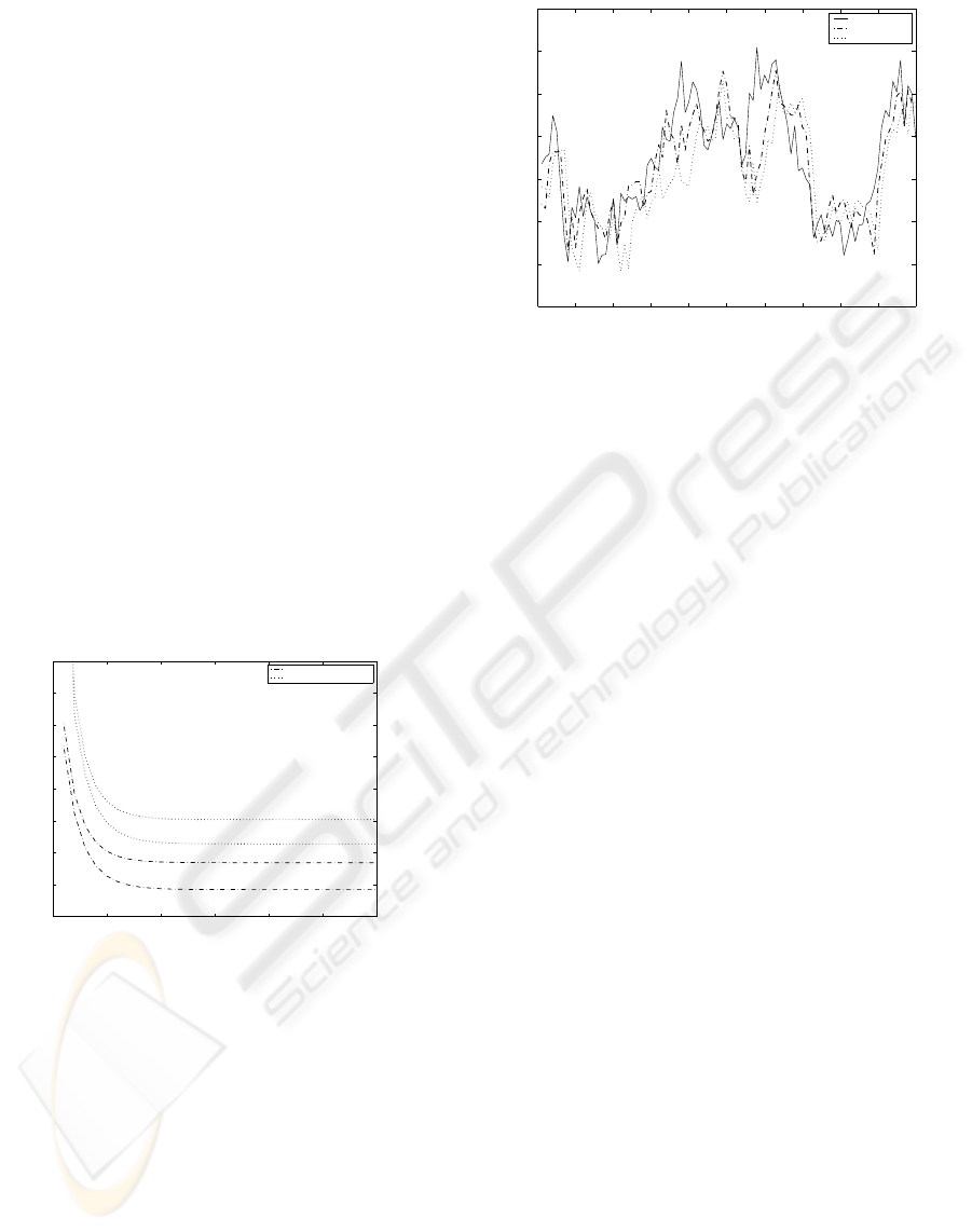
Finally, Figure 2 presents filtering estimates of
a simulated signal from delayed measurements for
p = 0.2 and p = 0.9. This figure shows that the
filter follows the signal evolution better as the delay
probability, p, is smaller, and, therefore, confirms the
comments about Figure 1.
5 CONCLUSION
In this paper, the linear one-stage predictor and filter
are derived from randomly delayed measurements
of the signal, for the case of white plus coloured
0 10 20 30 40 50 60 70 80 90 100
−1.5
−1
−0.5
0
0.5
1
1.5
2
Time k
Signal
Filter for p=0.2
Filter for p=0.9
Figure 2:Signal and filtering estimates for p = 0.2, 0.9
noises. It is assumed that the delay is modelled by a
sequence of independent Bernoulli random variables,
which indicate if the measurements arrive in time or
are delayed by one sampling period. The estimators
are obtained by an innovation approach and do not
require the knowledge of the state-space model of
the signal, but just the second-order moments of
the signal and noises, assuming a semi-degenerate
kernel form for the autocovariance functions of
the signal and the coloured noise, and the delay
probabilities. A numerical example shows that the
obtained algorithms are computationally feasible.
ACKNOWLEDGMENT
Supported by
the ‘Ministerio de Ciencia y Tecnolog
´
ıa’. Contract
BFM2002-00932.
REFERENCES
Evans, J. S. and Krishnamurthy, V. (1999). Hidden
Markov model state estimation with randomly
delayed observations. IEEE Transactions on Signal
Procesing, 47:2157–2166.
Matveev, A. S. and Savkin, A. V. (2003). Optimal computer
control via communication channels with irregular
transmission times. International Journal of Control,
76:165–177.
Nakamori, S., Caballero, R., Hermoso, A. and Linares,
J. (2004a). Fixed-interval smoothing from uncertain
observations with white plus coloured noises using
covariance information. IEICE Trans. Fundamentals,
E87-A, No. 5:1209–1218.
Nakamori, S., Caballero, R., Hermoso, A. and Linares,
J. (2004b). Recursive estimator of signals from
ICINCO 2004 - SIGNAL PROCESSING, SYSTEMS MODELING AND CONTROL
22

measurements with stochastic delays using covariance
information. Applied Mathematics and Computation,
(in press).
Yaz, E. and Ray, A. (1998). Linear unbiased state
estimation under randomly varying bounded sensor
delay. Applied Mathematics Letters, 11:27–32.
ESTIMATION ALGORITHM FROM RANDOMLY DELAYED OBSERVATIONS WITH WHITE PLUS COLOURED
NOISES
23
