
ON THE EFFICIENCY OF A CERTAIN CLASS OF NOISE
REMOVAL ALGORITHMS IN SOLVING
IMAGE PROCESSING TASKS
Catalina Cocianu
Academy of Economic Studies, Calea Dorobantilor 15-17, Bucharest #1, Romania
Luminita State
University of Pitesti, Caderea Bastiliei #45, Bucharest #1, Romania
Vlamos Panayiotis
Hellenic Open University, Greece
Viorica Stefanescu
Academy of Economic Studies, Calea Dorobantilor 15-17, Bucharest #1, Romania
Keywords: Noise removal, image processing, regression, filtering, multiresolution analysis, wavelet transform,
statistical image restoration techniques, least mean squares techniques
Abstract: The investigated noise removal algorithms are HRBA,
HSBA, HBA, AMVR, PNRA, MMSE, MNR,
MNR2 and NFPCA. The multiresolution support provides a suitable framework for noise filtering and for
restoration purposes by noise suppression. The techniques used in the paper are mainly based on the
statistically significant wavelet coefficients specifying the support. The performed tests reveal that the use
of the multiresolution support proves powerful and offers a versatile way to handle noise of different classes
of distributions.
1 INTRODUCTION
The restoration techniques are usually oriented
toward modeling the type of degradation in order to
infer the inverse process for recovering the original
image. Some of the techniques (HRBA, HSBA,
HBA, PNRA) presented in the sequel aim to
improve the quality of the filtered images using a
certain amount of information globally extracted
from the whole set of samples consisting of filtered
and non-filtered ones. The AMVR algorithm allows
the removal of the normal/uniform noise whatever
the mean of the noise is.
The multiresolution support provides a suitable
fram
ework for noise filtering and for restoration by
suppressing the noise. The MNR technique is
essentially based on the statistical significance of the
wavelet coefficients specifying the support.
An important feature of neural networks is the
ab
ility they have to learn from their environment,
and, through learning to improve performance in
some sense. In the following we restrict the
development to the problem of feature extracting
unsupervised neural networks derived on the base of
the biologically motivated Hebbian self-organizing
principle which is conjectured to govern the natural
neural assemblies and the classical principal
component analysis (PCA) method used by
statisticians for almost a century for multivariate
data analysis and feature extraction.
318
Cocianu C., State L., Panayiotis V. and Stefanescu V. (2004).
ON THE EFFICIENCY OF A CERTAIN CLASS OF NOISE REMOVAL ALGORITHMS IN SOLVING IMAGE PROCESSING TASKS.
In Proceedings of the First International Conference on Informatics in Control, Automation and Robotics, pages 320-323
DOI: 10.5220/0001127603200323
Copyright
c
SciTePress

2 ALGORITHMS FOR
IMPROVING THE QUALITY OF
FILTERED IMAGES
The research aimed the comparison of the
performances of our restoration algorithms HRBA,
HSBA, HBA, PNRA (Cocianu, 2002) and NFPCA
against well known algorithms that are currently
used for solving this type of problem.
Let X be the given image,
() ()
(
)
{
22
2
2
1
,...,,
N
XXX
}
a
sample of the
(
)
η+=
η
XX
, η~
(
)
Σ
µ
,N
and the sample of the filtered
random vector
() () ()
{
11
2
1
1
,...,,
N
XXX
}
()
(
)
η
XF
. Let
()
(
)
(
)()
η
=µ XFE
1
,
be the mean vectors and ,
() ()
(
η
=µ XE
2
)
11
Σ
22
Σ
the
covariance matrices. The HRBA is (State, 2001).
Step 1. Compute
() ()
(
)
{}
11
2
1
1
,...,,
N
XXX
by
applying the binomial filter to
() ()
(
)
{}
22
2
2
,...,,
N
XXX
ri ≤
1
.
Step 2. For each row
≤
1 , compute
()
()
()
()
2,1,
1
ˆ
1
==µ
∑
=
piX
N
i
N
k
p
k
p
()
()
()
()
()
()
()
()
()
()
(
2,1,
,
ˆˆ
1
1
ˆ
1
=
µ−µ−
−
=Σ
∑
=
st
iiXiiX
N
i
N
k
sss
k
tt
kts
)
Step 3. For each ri
≤
≤1 , compute
(
)
(
)
()
iT
1
ˆ
µ
by
applying a threshold filter to
()
()
i
1
ˆ
µ
Step 4. Compute
()
()
()
()
() ()
()
()
()
()
()
()
(
iiiiiTiX
12
2212
1
ˆˆ
ˆˆ
ˆ
µ−µΣΣρ+µ=
+
)
where
ρ is a noise-preventing suitable constant.
The HSBA is (State, 2001),
Step 1. Compute the sample
() ()
(
)
{
11
2
1
1
,...,,
N
XXX
}
as described in Step 1 of the HRBA
Step 2. For each
ri
≤
≤1 , do Step 3 until Step 7
Step 3. Compute
()
()
()
()
∑
=
=µ
N
k
p
k
p
iX
N
i
1
1
ˆ
,
2,1
=
p
()
()
()
()
()
()
()
()
()
()
(
∑
=
µ−µ−
−
=∑
N
k
T
pp
k
pp
kp
iiXiiX
N
i
1
ˆˆ
1
1
ˆ
)
Step 4. Compute
and
() () ()
iiiS
w 21
ˆˆ
∑+∑=
() ()
()
()
()
()
()
()
()
()
(
)
()
T
wm
iiiiiSiS
2121
ˆˆˆˆ
µ−µµ−µ+=
Step 5. Compute the eigenvalues
()
(
)(
ii
n
)
λ
λ ,...,
1
and the eigenvectors
() ()
(
)
ii
n
Φ
Φ
,...,
1
of
(
)
iS
m
.
Select the largest t eigenvalues and let
() () ()()
iidiagi
tt
λ
λ
,...,
1
=Λ ,
()
() ()
(
)()
iii
t
t
ΦΦ=Φ ,...,
1
()
()
() () ()
()
() ()
⎟
⎠
⎞
⎜
⎝
⎛
ΛΦ
⎟
⎠
⎞
⎜
⎝
⎛
ΛΦ=
−−
iiiSiiiK
t
t
w
T
t
t
2
1
2
1
Step 6. Compute
(
)
i
Ψ
the matrix having the
columns the unit eigenvectors of
. The most
informative features responsable for the class
separability are given by
()
iK
() () () ()
iiiiA
t
ΨΛΦ=
−
2
1
.
Step 7. Compute the row
()
iX
of the restored
image
X ,
(
)
iX
=
(
)
()
(
)
() ()
(
)
(
)
()
iTiAiAiT
11
ˆˆ
µσ+µ
+
,
where
σ
is a noise-preventing constant, 10
<
σ< .
The HBA image restoration algorithm is based on
the Bhattacharyya distance, (
State, 2001)
Step 1. Compute the sample
() ()
(
)
{}
11
2
1
1
,...,,
N
XXX
as described in Step 1 of HRBA
Step 2. For each
ri
≤
≤
1 , do Step 3 until Step 7
Step 3. Compute
()
()
()
()
∑
=
=µ
N
k
p
k
p
iX
N
i
1
1
ˆ
,
2,1
=
p
()
()
()
()
()
()
()
()
()
()
()
∑
=
µ−µ−
−
=∑
N
k
T
pp
k
pp
kp
iiXiiX
N
i
1
ˆˆ
1
1
ˆ
Step 4. Compute the Bhattacharyya distance
⎟
⎠
⎞
⎜
⎝
⎛
µ i,
2
1
.
Step 5 Compute the eigenvalues and
the eigenvectors
()
c
λλ ,...,
1
i
Φ
,
ci ,1
=
of .
() ()
ii
1
1
2
ˆˆ
∑∑
−
Step 6 Arrange the eigenvalues in the decreasing
order of
()
(
)
()
(
)
(
)
[
]
⎟
⎟
⎠
⎞
⎜
⎜
⎝
⎛
λ
+λ++
λ+
µ−µΦ
s
s
s
T
s
ii
1
2ln
1
ˆˆ
2
12
and
select the feature matrix
(
)( )
T
k
iM ΦΦ= ,...,
1
.
Step 7. Compute
(
)
=iX
(
)
(
)
(
)
() ()
()
()
()
iTiMiMiT
T 11
ˆˆ
µσ+µ
,
where
σ
is a noise-preventing constant, 0<
σ
<1.
The PNRA is based on the innovations algorithm
of the best linear predictors . Let X
0
be a R×C image,
R
≥
1, C
≥
1, whose pixels are colored on a N level
gray scale. We assume that the input is represented
by a sample {X
l
(1)
,l=1,...,n} on X
(1)
=X
0
+
η
(State,
2000). Using a binomial mask B and the contrast
enhancement operator P resulted by Lagrange
interpolation (Cocianu, 1997), we get the variants
X
(2)
=P(B(X
(1)
)), X
(3)
=P(X
(2)
). For each r=1,...,R and
c=1,...,C we define (State, 2000),
(
)
(
)
(
)
(
)
(
)
.3,2,1, =−= iXEXz
iii
Let {X
t
}
t
∈
Z
be a zero mean stochastic process,
K(i,j) its autocorrelation function and
,
⎩
⎨
⎧
≥
=
=
+
+
1,
0,0
1
1
nXP
n
X
nH
n
n
)
2
11
ˆ
++
−=
nnn
XXv
. If, for
any n
≥
1, [K(i,j)]
i,j=1,…,n
is a non degenerated matrix,
then we get (Brockwell, 1985)
ON THE EFFICIENCY OF A CERTAIN CLASS OF NOISE REMOVAL ALGORITHMS IN SOLVING IMAGE
PROCESSING TASKS
319

⎪
⎪
⎪
⎪
⎩
⎪
⎪
⎪
⎪
⎨
⎧
θ−++=
−=
⎟
⎠
⎞
⎜
⎝
⎛
θθ−++=θ
=
∑
∑
=
−
=
−−
−
−
k
j
j
jnn
n
k
j
jjnnjkkkknn
vnnKv
nk
vknKv
Kv
0
,
2
0
,,
1
,
0
)1,1(
1,0
,)1,1(
)1,1(
Aiming the removal of the residual noise, we apply
to each sample the transform,
()
nip
p
M
zz
i
ii
,1,1,1
3)4(
=>−+=
In order to develop an approximation scheme for
z
l
(4)
, l=1,...,n, we note that (State, 2000),
() () ()
∑
=
−α
−
+=
n
i
j
i
i
z
n
jKjK
1
)(
1
1
1
,3,4 ,
where
p
M
=α
. The description of the AMVR
algorithm is (Cocianu, 2002),
Input The
image Y representing a
normal/uniform disturbed version of the initial
image X,
,
CL ×
() ()
0
,
,,
cl
clXclY η+=
CcLl
≤
≤
≤≤ 1,1 ,
where is a sample of the random variable
0
,cl
η
cl,
η
distributed either
or .
()
2
,,
,
clcl
N σµ
()
2
,,
,
clcl
U σµ
Step 1. Generate the sample of images
, where
{}
n
XXX ,...,,
21
() ()
i
cli
clYclX
,
,, η−=
, CcLl ≤≤≤≤ 1,1
and
is a sample of the random variable
i
cl,
η
cl,
η
.
Step 2. Compute
() ()
∑
=
=
n
i
i
clX
n
clX
1
,
1
, , . CcLl ≤≤≤≤ 1,1
Step 3. Compute the estimation
X
ˆ
of X using the
adaptive filter MMSE,
()
XMMSEX =
ˆ
.
The multiresolution support provides a suitable
framework for noise filtering and for restoration
with noise suppression. The procedure used is to
determine statistically significant wavelet
coefficients and from this to specify the
multiresolution support, therefore a statistical image
model is used as an integral part of the image
processing. The support is used subsequently to
hand-craft the filtering processing. The MNR
algorithm is (Stark, 1995),
Input: The image
0
, the number of the
resolution levels p and the heuristic thresold k.
X
Step 1. Compute the image variants
{
}
pj
j
X
,1=
and
the wavelet coefficients using the “À Trous”
algorithm (Stark, 1995)
() ()
()
∑∑
−−
−
++=
lk
jj
jj
kclrXklhcrX
11
1
2,2,,
(
)
(
)(
crXcrXcr
jjj
,,,
1
)
−
=
ω
−
.
Step 2. Apply the test:
is significant if
and only if
(
cr
j
,ω
)
(
)
jj
kcr σ≥ω ,
, for
pj ,...,1=
Step 3. Compute the restored image,
.
() () ()
()
()
∑
=
ωωσ+=
p
j
jjjp
crcrgcrXcrX
1
,,,,,
~
In the following, we present a generalization of
the MNR algorithm based on the multiresolution
support set for noise removal in case of arbitrary
mean (Cocianu, 2003). Let g be the original “clean”
image,
η
~
(
)
2
,σmN
and the analyzed image
η
+
=
gf . The sampled variants of f, g and
η
obtained using the two-dimensional filter
ϕ
are
(
)
(
)
(
)
cylxclfyxc −−ϕ= ,,,,
0
,
(
)
(
)
(
)
cylxclgyxI −−ϕ= ,,,,
0
,
(
)
(
)
(
)
cylxclyxE −−ϕη= ,,,,
0
, .
000
EIc +=
The wavelet coefficients computed by the algorithm
“À Trous” are
(
)
yx
c
j
,
0
ω
()
(
)
yxyx
E
j
I
j
,,
00
ω+ω=
,
where
()
⎟
⎠
⎞
⎜
⎝
⎛
φ−φ=
⎟
⎠
⎞
⎜
⎝
⎛
ψ
22
1
22
1 x
x
x
. For any pixel
(
)
yx, , we get
(
)
yxc
p
,
() (
yxEI
pp
,yx, +=
)
)
.The
mean of the noise can be decreased using the
following algorithm.
Step1. Determine the images
, , by
superimposing noise sampled from
on the
“white wall” image.
()
i
E ni ≤≤1
(
2
,σmN
Step2. For all j,
pj
≤
≤
1
, compute ,
j
c
(
)
i
j
E ,
ni
≤
≤
1 and the coefficients using the “À
Trous” algorithm.
()
i
E
j
c
j
ωω ,
0
Step 3. Compute the image
I
~
by,
() ()
()
()
[
()
()
()
()
⎥
⎦
⎤
ω−ω+
+−=
∑
∑
=
=
p
j
E
j
c
j
n
i
i
pp
yxyx
yxEyxc
n
yxI
i
1
1
,,
,,
1
,
~
0
.
Step 4. Compute a variant of the original image
using the multiresolution filtering based on the
statistically significant wavelet coefficients.
0
I
An alternative approach in solving image
restoration task can be performed by PCA neural
network. The idea is to use features extracted from
the noise in order to compensate the lost information
and improve the quality of images. The NFPCA
algorithm is presented in the following. Let
0
I
be a
ICINCO 2004 - SIGNAL PROCESSING, SYSTEMS MODELING AND CONTROL
320
RxC matrix ( CnnCC <
≤
= 2,
1
) representing the
initial image of L gray levels and I the distorted
variant resulted from
0
I
by superimposing noise
, , ,
1
()
Σ,0N
Ri ,...,1=∀
()
njjnk ,...,1−= ,...,1 Cj
=
,
jiji
,,
. The restoration process of the
image I is described as follows.
() () ()
kkIkI η+=
0
Step 1. Compute the image I’ by decorrelating
the noise component,
,
~ ,
''
0
,,,
η+Φ=Φ=
ji
T
ji
T
ji
III
ηΦ=η
T
'
()
',0 ΣN Λ=
Σ
ΦΦ=Σ
T
' , where
{}
n
diag λλλ=Λ ,...,,
21
.
Step 2. The noise component is removed for
each pixel P of the image I’ using the
multirezolution support of I’ by the labeling method
of each wavelet coefficient of P, resulting I”.
'η
()
0
,,,
'"
ji
T
jiji
IIMSTI Φ≅=
,
Ri ,...,1=
∀
, .
1
,...,1 Cj =
Step 3. An approximation
0
~
I
I
≅
of the initial
image
0
I
is produced by applying the inverse
transform of
to I”.
T
T
Φ
3 COMPARATIVE ANALYSIS ON
THE PERFORMANCE OF THE
NOISE REMOVAL
ALGORITHMS
A series of experiments were performed, different
256 gray level images being preprocessed aiming the
contrast enhancement, increasing enlightens and
noise removing by filtering them. Our experiments
use the averaging and respectively binomial filtering
techniques. The parameters involved in the
mentioned algorithms were tuned taking into
account the following factors: the distortion degree
of the inputs, the particular smoothing filter, the
volume of the resulting accepted data (Cocianu,
2002).
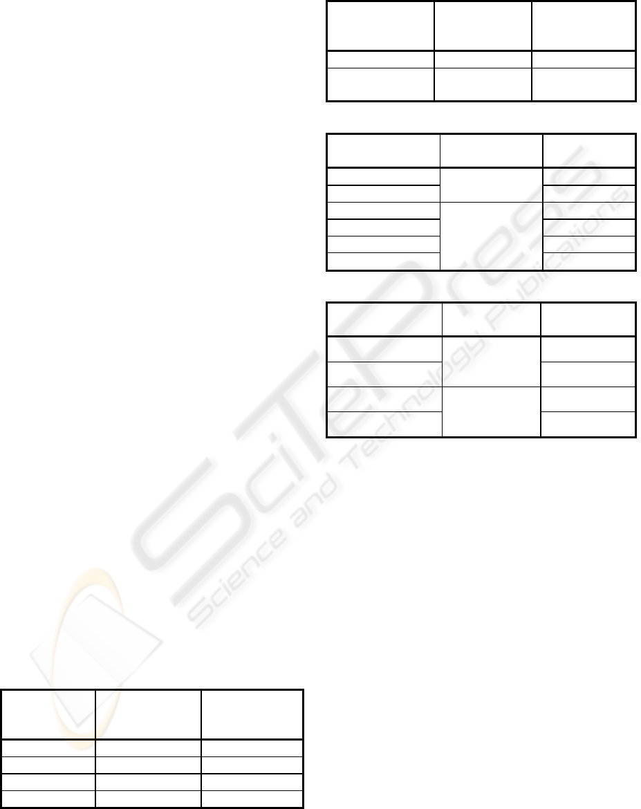
A synthesis of the comparative analysis on the
quality and efficiency corresponding to the
restoration algorithms presented in the paper is
supplied in Table 1, Table 2, Table 3 and Table 4.
Table 1
Restoration
algorithm
Mean
error/pixel
N(30,150)
Mean
error/pixel
N(50,200)
Mean 9.422317 12.346784
HRBA 9.333114 11.747860
HSBA 9.022712 11.500245
HBA 9.370968 11.484837
Table 2
Restoration
algorithm
Mean
error/pixel
N(50,200)
Mean
error/pixel
N(90,250)
Mean 12.346784 102.528893
The innovation
algorithm
11.647346 94.912895
Table 3
Restoration
algorithm
Type of
noise
Mean
error/pixel
MMSE 50.58
AMVR
U(40,70)
8,07
MMSE 46.58
AMVR 9.39
MNR2 12.23
NFPCA
N(50,100)
10.67
Table 4
Restoration
algorithm
Type of
noise
Mean
error/pixel
MNR
(
)
1
h
11.6
MNR
(
)
2
h
N(0,100)
9.53
MNR
(
)
1
h
14.16
MNR
(
)
2
h
N(0,200)
11.74
REFERENCES
Brockwell, P., Richard, A., 1985, Time Series: Theory
and Methods, Springer Verlag
Cocianu, C., State, L., Vlamos, P.,2002, On a Certain
Class of Algorithms for Noise Removal in Image
Processing: A Comparative Study, In Third IEEE
Conference on Information Technology ITCC-2002,
Las Vegas, Nevada, USA, April 8-10, 2002
Cocianu, C., State, L., Stefanescu, V., Vlamos, P., 2003,
Noise Removal Techniques Using the Multiresolution
Representation, In Proceedings of 32nd International
Conference on Computer&Industrial Engineering
(ICC&IE), Limerick, Ireland, August 11th-13th, 2003
Jain, A. K., Kasturi, R., Schnuck, B. G., 1995, Machine
Vision, McGraw Hill
Sonka, M., Hlavac, V., 1997, Image Processing, Analyses
and Machine Vision, Chapman & Hall Computing
Stark, J.L., Murtagh, F., Bijaoui, A., 1995, Multiresolution
Support Applied to Image Filtering and Restoration,
Technical Report
State, L, Cocianu, C, Vlamos, P.., 2001, Attempts in Using
Statistical Tools for Image Restoration Purposes, In
Proceedings of SCI2001, Orlando, USA, 2001
ON THE EFFICIENCY OF A CERTAIN CLASS OF NOISE REMOVAL ALGORITHMS IN SOLVING IMAGE
PROCESSING TASKS
321
