
PARAMETRIC ESTIMATION OF SINUSOIDS IN NOISE
A comparison between parametric approaches and the definition of a regularized
Smyth algorithm
Aldo Balestrino, Andrea Caiti and Roberto Mati
DSEA – Dept. Electrical Systems and Automation, University of Pisa, Italy
Keywords: Estimation, sinusoids, signals, parametric algorithms
Abstract: A comparison between well-established parametric algorithms and the more recent Smyth algorithm for
estimation of sin
usoidal signals in white noise is presented. The comparison is performed through a pseudo-
Monte Carlo analysis on simulated data. The results obtained show that Smyth algorithm has a slightly
better performance at large Signal-to Noise Ratios. However, when the SNR drops down, the performance
of the Smyth algorithm dramatically decreases. A better performance with respect to both ESPRIT and
Smyth algorithms at low SNR can be obtained by a regularized filtering procedure on the data.
1 INTRODUCTION
The detection of sinusoidal signals embedded in
noise is a classic problem, of wide interest in
numerous applications, from sonar to radar and
tracking problems. The available algorithms can be
classified as parametric and non parametric methods.
The non parametric methods are based on classical
periodogram analysis (Stoica and Moses, 1997).
Parametric methods include Auto Regressive (AR) –
based algorithms and high resolution eigenanalysis
approaches.
Popular eigenanalysis algorithms include MUSIC
(Sc
hmidt, 1983), ESPRIT (Roy and Kailath, 1989)
and the classic Pisarenko algorithm (Pisarenko,
1973). More recently, Smyth has proposed a novel
eigenanalysis algorithm by combining a constrained
Pisarenko approach with an iterative least square
estimator (Smyth, 2000).
The purpose of this paper is to compare the above
m
entioned algorithms at different Signal to Noise
Ratios (SNR), in order to evaluate pros and cons of
the various approaches. The comparison is done
through a pseudo Monte Carlo method on simulated
data. The results obtained show that the Smyth
algorithm has a slightly better performance with
respect to the other methods at high SNR. At low
SNR, with specific values depending on the number
of different sinusoids to be estimated, MUSIC and
ESPRIT seems to yield the best performance.
The comparison reported is in itself interesting
an
d valuable, since to the Authors knowledge no
comparison of the traditional methods with the
Smyth approach has appeared in the literature. In
addition to that, the above results have also led to the
definition of a novel estimation algorithm. The novel
approach is essentially an iterated application of the
Smyth algorithm to a succession of regularized data
set. The regularization is obtained as a weighted sum
of the predicted, noise-free data from the previous
step solution with the noise-corrupted
measurements. The data weighting depends on a
regularization parameter which is changed from step
to step in order to reach, in a finite number of steps,
the situation in which the algorithm uses only the
data measurements. The initialization of this filtering
procedure is done with the predicted, noise free
solution obtained from ESPRIT. By using the
simulative approach which has been employed for
the algorithms comparison, it is shown that there
does exist an optimal value of the regularization
parameter such that for this value the proposed
algorithm has performance better than both ESPRIT
and Smyth algorithms.
The paper is organized as follows. In the next
section, a formal state
ment of the problem is given
and the Smyth algorithm is briefly reviewed. In
section 3 the simulative trials and the results
obtained by comparing the performance of ESPRIT,
MUSIC, Pisarenko and Smyth algorithms are
reported. In section 4 the novel regularization
algorithm is presented, and the existence of an
299
Balestrino A., Caiti A. and Mati R. (2004).
PARAMETRIC ESTIMATION OF SINUSOIDS IN NOISE - A comparison between parametric approaches and the definition of a regularized Smyth
algorithm.
In Proceedings of the First International Conference on Informatics in Control, Automation and Robotics, pages 301-306
DOI: 10.5220/0001128103010306
Copyright
c
SciTePress

optimal continuation parameter is enlightened. In
section 5, some comments on the computational
burden of the various approaches are given, and
future efforts in order to determine algorithmically
the optimal parameter are briefly described. Finally,
some conclusions are given.
2 THE SMYTH PROBLEM AND
THE SMYTH ALGORITHM
It is supposed to have available the measurements:
Kkkwksky
n
j
j
,...,1 , )()()( =+=
∑
(1)
where
are the samples of n
sinusoidal signals, each at the frequency
njks
j
,...,1 ),( =
ji
ijj
≠≠ if ,
ω
ω
ω
, and is a finite power
white process uncorrelated with the sinusoidal
signals. Given the measurement of
K samples of the
output signal
, and given the knowledge of the
number
n of frequencies present in the measurement,
the problem is to obtain an estimate of the
frequencies
)(kw
)(ky
nj
j
,...,1 , =
ω
.
The following estimation procedure has been
introduced by Smyth (Smyth, 2000). The procedure
is composed of three steps. In the first one, a
constrained Pisarenko algorithm is applied. The
estimate thus obtained is used as starting point of the
second step, in which the Osborne-Bresler-
Makovsky (OBM) estimation algorithm is applied
(Bresler and Makovsky, 1986). Finally, the results of
the second step are used to initialize a least square
iterative estimation (Osborne, 1975). The idea
behind the Smyth approach is that the three
algorithms, Pisarenko, OBM and Osborne, are
applied in order of increased sensitivity to the
initialization. So, the least sensitive to the initial
condition is applied as first, while the others are
used to progressively refine the solution.
Formally, let
be the auto correlation matrix of
the measurement signal
; let be the
eigenvector associated to the smallest eigenvalue of
, and let:
Y
)(ky
c
Y
n
n
zczcczc
2
210
...)( ++=
be the annihilator polynomial whose coefficients are
given by the components of
c
. By observing that
and must have the same roots, Smyth
has introduced a constrained Pisarenko estimate for
the eigenvector
in the following iterative form: at
each iteration
it must be solved the constrained
least square problem:
)(zc )(
1−
zc
c
h
)1()()1(
1
)( min
++
=
hh
T
h
D
T
cY cc
cc
(2)
where
D is a matrix imposing the root constraint.
Equation (2) is successively solved by Pisarenko,
OBM and Osborne least-square algorithms, using as
starting point the solution obtained in the previous
step.
3 SIMULATIVE EVALUATION OF
THE SMYTH ALGORITHM
In this section a pseudo Monte Carlo simulative
study is presented, reporting the performance
obtained by the Smyth algorithm as compared with
the standard Pisarenko, MUSIC and ESPRIT
algorithms. Results from a non-parametric, FFT-
based, estimation algorithm are also reported. Three
cases are considered. In the first, the signal is
assumed to be composed by a single sinusoid, in the
second by two and in the third by four sinusoids, all
added up with random phases. Gaussian white noise,
is added to the signal, with varying Signal-to-Noise
Ratio (SNR), from –20 up to 40 dB, at 2.5 dB steps.
All simulations have been carried out in Matlab
environment, version 6.5. In each trial, performances
are obtained as follows. For each algorithm, and for
each SNR the signal
y(k) is generated as the sum of
the predefined number of tones plus noise. Then all
the algorithms are applied to
y(k). Such a procedure
is repeated
N = 100 times. The estimated Mean
Square Error from each algorithm is computed as
follows:
()
(
)
∑
=
−=
N
i
j
i
jj
N
MSE
1
2
)(
ˆ
1
ωωω
(3)
∑
=
=
n
j
j
MSEMSE
1
)(
ω
(4)
where
is the estimate of the j-th frequency in
the
i-th run.
j
i)(
ˆ
ω
In the figures reported in the following, the
value in dB of 1/MSE is plotted as a function of the
SNR, so that for each SNR, the higher the y-scale
value, the better is the performance for each
algorithm. Numerically, a normalized sampling time
of 1 second has been used, with a window of K=300
samples. The chosen frequencies have been taken as
1
ω
= 0.025 Hz,
2
ω
= 0.062 Hz,
3
ω
= 0.1021 Hz,
4
ω
= 0.2848 Hz.
ICINCO 2004 - SIGNAL PROCESSING, SYSTEMS MODELING AND CONTROL
300
-20 -10 0 10 20 30 40
0
20
40
60
80
100
120
SNR (dB)
1/MSE (dB)
FFT
Pisarenko
MUSIC
ESPRIT
Smyth
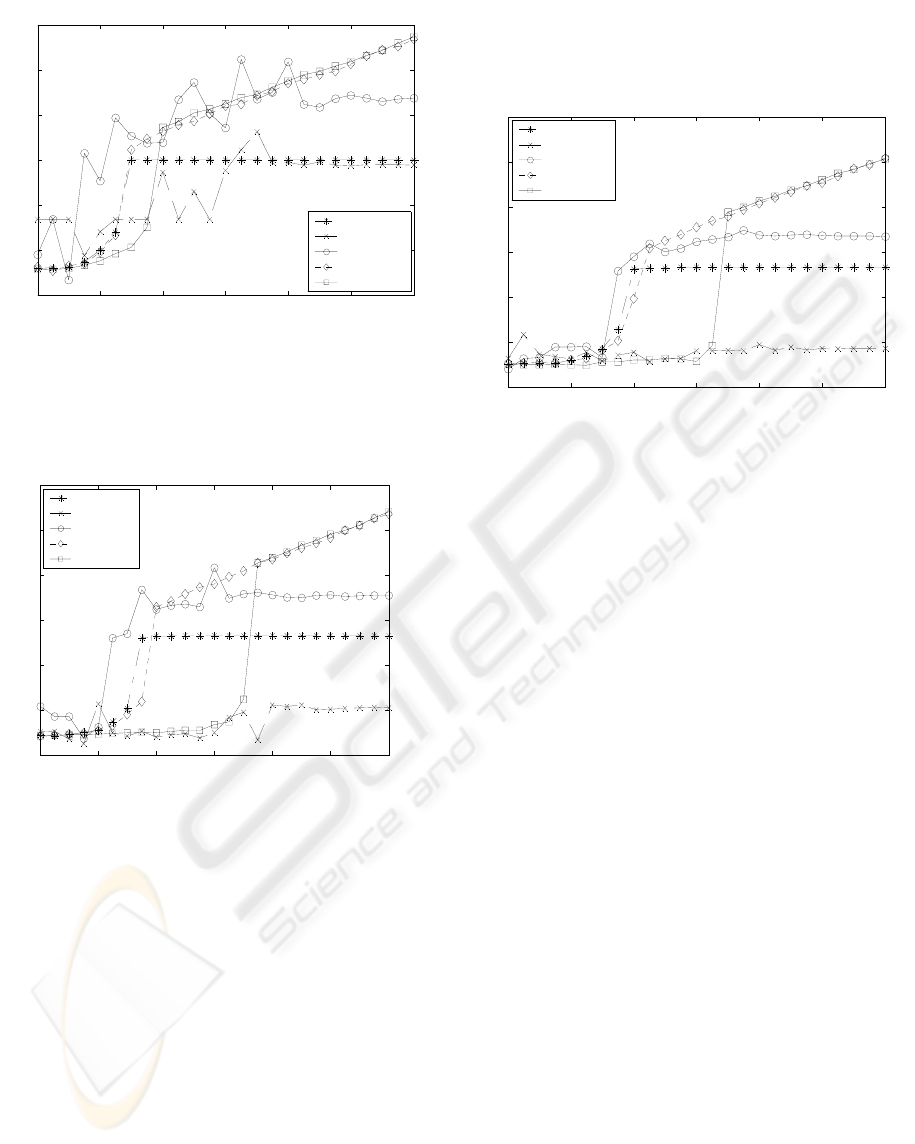
Figure 1: Performance results from pseudo Monte Carlo
analysis for the estimation of a single frequency. dash-dot
line: FFT; dashed, with crosses: Pisarenko; continuous
line, with circles: MUSIC; dotted line, with diamonds:
ESPRIT; continuous line with squares: Smyth.
-20 -10 0 10 20 30 40
0
20
40
60
80
100
120
SNR (dB)
1/MSE (dB)
FFT
Pisarenko
MUSIC
ESPRIT
Smyth
Figure 2: Performance results from pseudo Monte Carlo
analysis for the simultaneous estimation of two
frequencies; dash-dot line: FFT; dashed, with crosses:
Pisarenko; continuous line, with circles: MUSIC; dotted
line, with diamonds: ESPRIT; continuous line with
squares: Smyth.
In figures 1, 2 and 3 the results obtained in the
estimation of one, two and four sinusoids
respectively are reported.
The results reported show that, at high SNR, the
Smyth approach can lead to some slight
improvement (few dB at the best) with respect to
ESPRIT, which has the best performance among the
standard methods. At low SNR, the performance of
Smyth algorithm drops down quite dramatically;
moreover, at low SNR MUSIC becomes competitive
with ESPRIT, succeeding in obtaining the best
performance in some cases. The behaviour of
MUSIC as a function of the SNR, however, is less
predictable with respect to that of the other methods,
and of ESPRIT in particular, showing weak
correlation among the algorithm performance at
varying SNR.
-20 -10 0 10 20 30 40
0
20
40
60
80
100
120
SNR (dB)
1/MSE (dB)
FFT
Pisarenko
MUSIC
ESPRIT
Smyth
Figure 3: Performance results from pseudo Monte Carlo
analysis for the simultaneous estimation of four
frequencies. dash-dot line: FFT; dashed, with crosses:
Pisarenko; continuous line, with circles: MUSIC; dotted
line, with diamonds: ESPRIT; continuous line with
squares: Smyth.
4 SMYTH ESTIMATION WITH
REGULARIZED DATA
The results presented in the previous section have
led to the exploration of a novel procedure in which
the Smyth algorithm is applied to a filtered,
regularized version of the data. The starting
motivation was to increase the performance of the
Smyth algorithm by increasing the SNR by a
process-guided data filtering. As a result, as it will
be shown in the following, a consistent improving in
the performance can be obtained. The proposed data
regularization procedure is the following: the filtered
data are obtained as a weighted sum of the predicted,
noise free data obtained from an estimated solution
(by whatever method) and the noise-corrupted
measurements. In order to generate the noise free
predicted data
, one has to start from the
estimated frequencies; keeping fixed these
frequencies it is possible, through standard Fourier
analysis, to estimate also the phase and amplitude of
these frequency components. This estimate leads to
the estimate
of the time series (1) without the
noise components. The regularized data set is then
obtained as:
)(
ˆ
ky
)(
ˆ
ky
)(
ˆ
)1()()( kykyky
a
α
α
−
+
=
(5)
where
10
≤
≤
α
is the regularization parameter,
trading off between measurement fidelity and
PARAMETRIC ESTIMATION OF SINUSOIDS IN NOISE - A COMPARISON BETWEEN PARAMETRIC
APPROACHES AND THE DEFINITION OF A REGULARIZED SMYTH ALGORITHM
301
confidence in the estimate. When
0=
α
the filtered
data are equal to the prediction (complete confidence
in the estimate), when
1
=
α
no filtering is applied
to the measurement.
In applying the Smyth algorithm to the filtered
data of equation (5) one has to select the
regularization parameter. In order to investigate the
algorithm performance as a function of the
regularized parameter, the following procedure has
been applied: the regularization parameter
α
is
made varying from 0 to 1 in
1+h steps:
0
0
=
α
, hh
h
hh
,...,1,
1
1
=+=
−
αα
,
1
=
h
α
The noise free predicted data
from
the estimate obtained with parameter
1−h
)(
ˆ
1
ky
h−
α
α
are used
to generate the filtered data with parameter
h
α
,
accordingly to the equation:
)(
ˆ
)1()()(
1
kykyky
h
ahh
h
a
−
−+=
α
α
(6)
The Smyth algorithm is applied to this data; then
its results are used to compute a new data prediction,
and the procedure is iterated. The Smyth algorithm
is also intialized with the solution obtained at the
previous step. Substantially, the algorithm is
successively applied to convex combinations of
noise-free data estimates obtained from the previous
step estimation and measurements The procedure is
initialized at step 0 with the ESPRIT algorithm,
whose data prediction is employed to compute the
regularized data with
0
=
α
. The same procedure
described in the previous section has then been
applied to evaluate the performance of the Smyth
algorithm as a function of the regularization
parameter. The results presented report the value in
dB of 1/MSE (equation (4)) against the value of
α
from 0 to 1, at 0.1 steps. The maximum corresponds
to the optimal regularization parameter. The two
limit cases corresponds to the independent
application of ESPRIT (
0=
α
) and Smyth ( 1
=
α
)
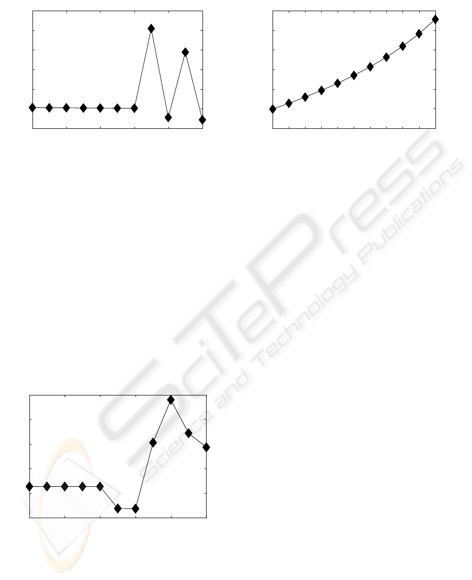
algorithms. A sample of the results obtained are
reported in Figures 4, 5, 6: the figures refer to the
estimation of two sinusoids, at SNR of –5, -10, -20
dB respectively. The results reported show the
existence of an optimal value of the regularization
parameter; the Smyth algorithm, applied with the
initialization process described and with the optimal
regularization parameter, has a performance at low
SNR which is better than that of both the "pure
Smyth" algorithm and ESPRIT. The average
performance gain with respect to ESPRIT of the
regularization approach ranges from the 8 dB of the
–10 dB SNR case (Figure 5) to the 3 dB of the –20
dB SNR case (Figure 6). Note that the performance
gain with respect to the "pure Smyth" algorithm can
be much larger (up to 45 dB, Figure 4). This general
behaviour is systematic in all the simulations test
performed, with sometimes even larger performance
gains.
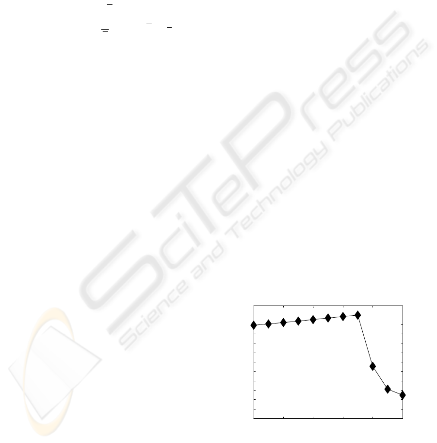
It is natural to ask what is the optimal
regularization parameter at high SNR. A typical
behaviour is shown in Figure 7, obtained in the case
of estimation of a single tone with SNR of 30 dB:
the optimal value is 1, indicating that the best
performance is given by the unregularized Smyth
algorithm.
It needs to be observed, though, that the
performance curve as a function of the regularization
parameter as determined through the pseudo Monte
Carlo approach does not exhibit any specific
behaviour that can be further exploited. In particular,
Figures 4-6 has been purposely chosen to illustrate
the several different behaviours observed. Figure 4
illustrates the situation in which the experimental
curve exhibits a unique maximum, with monotone
behaviour of the performance curve before and after
the extremal point; Figure 5 shows the presence of
multiple maxima and minima; Figure 6 presents a
case in which, though there does exist a unique
maximum, there is also a minimum within the
regularization interval, and the performance function
does not have a monotone behaviour before the
reaching of the maximum. Moreover, for some
values of the regularization parameter, the
performance is worse with respect to both ESPRIT
and unregularized Smyth. This diversity in the
performance curve behaviour may represent a
serious obstacle to an efficient implementation of a
computational scheme aimed at exploiting the better
performance of the regularized approach. Some
guidelines and critical evaluations toward this goal
are reported in the next section.
0 0.2 0.4 0.6 0.8 1
0
5
10
15
20
25
30
35
40
45
50
55
60
1/MSE (dB)
regularization parameter
SNR = -5 dB
2 sinusoids
Figure 4: Estimation results obtained from the Smyth
algorithm and the regularization procedure as a function of
the regularization parameter; SNR: -5 dB.
ICINCO 2004 - SIGNAL PROCESSING, SYSTEMS MODELING AND CONTROL
302
0 0.2 0.4 0.6 0.8 1
12
14
16
18
20
22
24
1/MSE (dB)
regularization parameter
SNR: -10 dB
2 sinusoids
Figure 5: Estimation results obtained from the Smyth
algorithm and the regularization procedure as a function of
the regularization parameter: SNR: -10 dB.
5 REGULARIZED ALGORITHM:
COMPUTATIONAL ASPECTS
The results reported in section 4 seems promising:
they establish the existence of a regularized Smyth
procedure through which a performance gain of
several dB with respect to ESPRIT can be obtained
by the proper selection of the regularization
parameter. This may lead to a substantial
improvement of the performance curves (Figures 1-
3) at low SNR, where the drop in performance had
been observed. On the other hand, there are some
non trivial computational aspects to be discusses
before the regularization approach can be
successfully implemented in a real life situation.
Figure 6: Estimation results obtained from the Smyth
algorithm and the regularization procedure as a function of
the regularization parameter: SNR: -20 dB
0 0.1 0.2 0.3 0.4 0.5 0.6 0.7 0.8 0.9 1
78
80
82
84
86
88
90
1/MSE (dB)
regularization parameter
SNR = 30 dB
1 sinusoid
Figure 7: Estimation results obtained from the Smyth
algorithm and the regularization procedure as a function of
the regularization parameter: SNR: 30 dB.
In particular, the performance curves of Figures
4-6 have been determined with the knowledge of the
true solution, which of course is never available in
practice. A practical implementation may consist in
repeatedly applying the algorithm varying the
regularization parameter over the whole admissible
range, and looking for the best performance by
comparison of the predicted time series with the
measured time domain data. How this is best
accomplished (by direct residual minimization, by
whiteness test on the residual time series, etc.) it is
not clear at the moment. Some preliminary tests with
the residual mean square error show both light and
shadows: in Figure 8 the time domain MSE is
plotted as a function of the regularization parameter
(as before, the plot refers to the quantity 1/MSE in
dB). Figure 8 correspond to the case reported in
Figure 6: -20 dB SNR and 2 unknown sinusoids.
The performance curve measured on the residual in
time domain has the maximum in correspondence of
the same regularization parameter as determined in
the frequency domain with the knowledge of the true
solution; however, the two performance curves do
not have the same behaviour, so that a systematic
exploitation of the time domain curve may also lead
to inaccuracies or undetected mistakes. Additional
considerations are related to the computational
burden of the Smyth approach, either in its "pure"
or regularized version, with respect to the attainable
performance gain. In Table 1 the mean computation
time of ESPRIT and of the Smyth algorithm, taken
over the 100 simulations described in Section 3, are
reported. The computation time refers to our Matlab
implementation running on a Pentium 4 PC, 2.4
GHz clock, under Windows XP operating system.
0 0.2 0.4 0.6 0.8 1
10
11
12
13
14
15
1/MSE (dB)
regularization parameter
SNR: -20 dB
2 sinusoids
PARAMETRIC ESTIMATION OF SINUSOIDS IN NOISE - A COMPARISON BETWEEN PARAMETRIC
APPROACHES AND THE DEFINITION OF A REGULARIZED SMYTH ALGORITHM
303

Table 1: comparison between ESPRIT and Smyth
algorithm computation times
Mean computation time (ms)
1 freq. 2 freq. 4 freq.
ESPRIT 9.9 10.2 8.5
SMYTH 41.6 77.4 105.4
The regularized Smyth algorithm consists of the
successive application of several Smyth algorithms,
with in addition the computational effort of
computing the new data set through Equation (6). So
there may as well be a factor of 100 in the
computational speed in favour of ESPRIT.
6 CONCLUSIONS
The paper has concentrated on two main topics: a
pseudo Monte Carlo evaluation of standard
parametric algorithms with respect to the Smyth
algorithm; an investigation of an innovative
regularization technique to improve the performance
of the Smyth algorithm at low SNR. The evaluation
study has shown that the Smyth algorithm can lead
to a slightly better performance with respect to
ESPRIT (the best among the standard parametric
algorithms tested) at high SNR. The Smyth
performance drops down dramatically at low SNR,
with a SNR threshold that is higher the greater the
number of sinusoids to be estimated. It has been
shown that, with the regularization approach
introduced, the Smyth algorithm is capable to
improve consistently its performance at low SNR,
with respect to its own performance, and also with
respect to ESPRIT. In particular, performance gains
up to 10 dB have been obtained. The results reported
are an experimental verification of the existence of
an optimal regularization parameter. Steps toward
the definition of an algorithm for the search of the
optimal parameter have been reported, as well as the
computational issues to be taken into account.
0 0.2 0.4 0.6 0.8 1
10
11
12
13
14
15
1/MSE (dB)
regularization parameter
SNR: -20 dB
2 sinusoids
Figure 8: Performance results computed from the time
domain residual as a function of the regularization
parameter: SNR: -20 dB
REFERENCES
Bresler, Y., Macovsky, A., 1986. Exact maximum
likehood parameter estimation of superimposed
exponential signals in noise.
IEEE Trans. Acoustic,
Speech, Signal Processing
, vol. 34, pp.1081-1089.
Osborne M.R., 1975. Some special nonlinear least square
problems.
SIAM J. Numer. Anal., vol. 12, pp.571-592.
Pisarenko, V.F., 1973. The retrieval of harmonics from
covariance functions,
Geophys. J. R. Astr. Soc., vol.
33, pp.347-366.
Roy, R., Kailath T., 1989. ESPRIT – Estimation of signal
parameters via rotational invariant techniques,
IEEE
Trans. Acoust. Speech Sig. Proc.
, vol. 37, pp. 984-995.
Schmidt R.O., 1983. A signal subspace approach to
multiple emitter location and spectral estimation,
Ph.D. thesis, Stanford University, Stanford, CA.
Smyth G.K., 2000. Employing symmetry constraints for
improved frequency estimation by eigenanalysis
methods,
Technometrics, n. 42, pp. 277-289.
Stoica, P., and Moses, R., 2000.
Introduction to spectral
analysis
, Prentice-Hall.
ICINCO 2004 - SIGNAL PROCESSING, SYSTEMS MODELING AND CONTROL
304
