
HIERARCHICAL MODAL CONTROL OF A NOVEL
MANIPULATOR
Clarence W. de Silva, Jian Zhang
Department of Mechanical Engineering, University of British Columbia, Vancouver, BC, Canada
Keywords: Deployable manipulator, Intelligent tuning, Modal control
Abstract: This paper focuses on the development and implementation of an intelligent hierarchical controller for the
vibration control of a deployable manipulator. The emphasis is on the use of knowledge-based tuning of the
low-level controller so as to improve the performance of the system. To this end, first a fuzzy inference
system (FIS) is developed. The FIS is then combined with a conventional modal controller to construct a
hierarchical control system. Specifically, a knowledge-based fuzzy system is used to tune the parameters of
the modal controller. The effectiveness of the hierarchical control system is investigated through numerical
simulation studies. Examples are considered where the system experiences vibrations due to initial
disturbance at the flexible revolute joint or due to maneuvers of a deployable manipulator. The results show
that the knowledge-based hierarchical control system is quite effective in suppressing vibrations induced
due to the above mentioned disturbances. Results suggest that performance of the modal controller could be
significantly improved through knowledge-based tuning.
1 INTRODUCTION
Among the fundamental developments in the
modern control theory are the two sets of analytical
results that underlie the linear quadratic regulator
(LQR) and eigenstructure assignment regulator
(EAR). Design and implementation of practical
control of flexible structures have been
accomplished using both the design techniques
(Junkins, 1993). In the LQR approach, the central
feature is the minimization of a quadratic
performance index, subject to a linearized system
model. However, a major drawback of the LQR is
that it has no direct control of the system
eigenstructure, which determines not only the level
of stability but also the specific nature of the
response to a control input (e.g., a step function).
The LQR method does not involve the assignment of
the system eigenstructure in a specified manner.
Consequently, it is desirable to employ a control
strategy that has the capability to modify the system
eigenstructure appropriately to meet specified
requirements. Such a control approach would prove
more effective if the capability of the parameter
tuning is available as well. To this end, a modal
control strategy is introduced here. An intelligent
control system, which combines a modal controller
and a fuzzy tuning structure, is developed to
‘intelligently’ assign the system eigenstructure so as
to obtain better performance of the controller in
terms of response speed, overshoot, and steady state
offset. Simulation studies have been carried out
using this intelligent control system to suppress
vibrations of a ground-based deployable
manipulator. The approach may be conveniently
applied to a space-based manipulator as well.
2 CONTROL SYSTEM
DEVELOPMENT
2.1 Eigenvalue Assignment
A linear system may be expressed in the state-space
form as
L
LL
=
+xAxBu
&
, (1)
where the time-dependent state vector
L
x
contains
generalized coordinates and their first time
derivatives of the system. The square matrix A is
composed of the matrices of mass, damping and
stiffness. The term B
L
u
(t) represents the effect of a
control action, with
L
u (t) and B being the control
force (torque) vector and actuator placement matrix,
206
de Silva C. and Zhang J. (2004).
HIERARCHICAL MODAL CONTROL OF A NOVEL MANIPULATOR.
In Proceedings of the First International Conference on Informatics in Control, Automation and Robotics, pages 206-213
DOI: 10.5220/0001128302060213
Copyright
c
SciTePress

respectively. As is normally the case in such studies,
all states are assumed to be available thus making
the system observable. By introducing state
feedback, the control input u
L
can be written as
L
L
=−uKx
. (2)
Thus one obtains a closed loop system
(- )
L
L
=xABKx
&
. (3)
In Equation (3), matrix
-
A
BK decides the
modal parameters of the closed loop system, such as
the modal frequencies, damping ratios and mode
shapes. A relation exists, between the modal
parameters of the system and the eigen-parameters
of matrix
A-BK, as eigen-parameters decide the
controlled behavior of the closed loop system
(Nishitani,1998), Equation (3). To obtain the relation
explicitly, it is useful to define some notations.
Assuming
A-BK to be a matrix of real-numbers, the
eigenvalues and eigenvectors of
A-BK appear as
conjugate pairs. Let
21i
λ
−
and
2i
λ
be the ith pair of
eigenvalues, and
21i−
z
and
2i
z
be the corresponding
ith pair of eigenvectors. Also let
,
ii
ωζ
and n
i
denote, respectively, the modal frequency, damping
ratio and mode shape of the
ith mode. Then we have:
2
21
2
2
j1
j1- ;
iiiii
iiiii
λζωωζ
λζωωζ
−
=− + −
=− −
;
⎫
⎬
⎭
and
21 2
21 2
;
ii ii
ii
ii
λλ
−
−
⎧⎫ ⎧
==
⎨⎬ ⎨
⎩⎭ ⎩
nn
zz
nn
;
for
i = 1 to n , (4)
where j =
1−
, and n is the number of degrees of
freedom of the system.
Equation (4) gives a one-to-one mapping
between the system modal parameters and the eigen-
parameters of matrix A
-BK. Therefore, if the modal
parameters
,i
and
ii
ωζ
n
are specified in the
domain, one can calculate the corresponding
eigenvalues and eigenvectors for the closed loop
system using Equation (4). Moreover, according to
Equation (3), if one can modify and assign the
eigenstructure at desired values by selecting proper
feedback matrix K, the modal property of the system
can be modified accordingly. This is the essence of
the modal control procedure. It is also the reason
why modal control is also called eigenvalue
assignment control.
2.2 Hierarchical Structure
The control system developed for the deployable
manipulator system has a three-level structure. This
hierarchical form combines the advantages of a crisp
controller, i.e. a modal controller, with those of a
soft, knowledge-based, supervisory controller. The
overall structure can be developed into three main
layers (de Silva, 1995).
Bottom Layer
The bottom layer deals with information coming
from sensors attached to the system. This type of
information is characterized by a large amount of
high resolution data points produced and collected at
high frequency. The crisp controller used is a state
feedback regulator with feedback gain matrix
determined using the eigenstructure assignment
approach. The control algorithm can be described as:
;
- ;
=
+
=
xAxBu
uKx
&
(5)
where u is the control action and K the feedback
matrix.
Intermediate Layer
The data processing for monitoring and
evaluation of the system performance occurs in the
intermediate layer. Here high-resolution, crisp data
from sensors are filtered to allow representation of
the current state of the manipulator. This servo-
expert layer acts as an interface between the crisp
controller, which regulates the servomotors at the
bottom layer, and the knowledge-based controller at
the top layer. The intermediate layer handles such
tasks as performance specification, response
processing, and computation of performance indices.
This stage involves, for example, averaging or
filtering of the data points, and computation of the
rise time, overshoot, and steady state offset.
Top Layer
The knowledge base and the inference engine in
the uppermost layer are used to make decisions that
achieve the overall control objective, particularly by
improving the performance of low-level direct
control. This layer can serve such functions as
monitoring the performance of the overall system,
assessment of the quality of operation, tuning of the
low-level controllers, and general supervisory
control. In this layer, there is a high degree of
information fuzziness and a relatively low control
bandwidth. Figure 1 presents the hierarchical
structure of the three-level control system.
HIERARCHICAL MODAL CONTROL OF A NOVEL MANIPULATOR
207

2.3 Performance Specification,
Evaluation, and Classification
The desired performance of the system is specified
in terms of the following time domain parameters:
• Rise time ( );
d
RST
• Overshoot, if underdamped ( );
d
OVS
• Offset at steady state ( ).
d
OFS
These three parameters are used to present the
desired performance of the system. The rise-time is
chosen as the time it takes for the response to reach
95% of the desired steady-state response. The
overshoot is calculated at the first peak of the
response. The steady-state offset is computed by
taking the difference between the average of the last
third of the response and the desired response.
The corresponding time domain parameters are
obtained from the response of the actual system,
with the subscript
r referring to the real system
response as:
, , and . Once
evaluated, the parameters of the real system are
compared with the desired ones to get the index of
deviation. For each performance attribute, an index
of deviation is calculated using the following
equation,
r
RST
r
OVS
r
OFS
Index of deviation of attribute = 1
−
th
i
th
th
i desired attribute
i actual attribute
(6)
The index is defined in such a way that the value of
1 corresponds to the worst-case performance, while
zero means the actual performance of the system, for
that particular attribute, exactly meets the
specification. The indices are calculated according
to:
1(
d
i
r
RST
RST ERR
RST
=− = 1)
; (7)
1
d
i
r
OVS
OVS ERR
OVS
=− =
(2)
; (8)
1
d
i
r
OFS
OFS ERR
OFS
=− =
(3)
. (9)
These indices represent the performance of the
system and hence should correspond to the context
of the rulebase of system tuning. The index of
deviation is therefore fuzzified into membership
values according to the five selected primary fuzzy
states: Highly Unsatisfactory (HIUN), Needs
Improvement (NDIM), Acceptable (ACCP), In
Specification (INSP) and Over Specification
(OVSP). In order to obtain a discrete set of
performance indices K(i), threshold values TH(i) are
defined for each index of deviation over the interval
-
∞
to 1, as given in Table 1.
Table 1: Mapping from the index of deviation to a discrete
performance index
The performance indices obtained in this
manner are the input to a Fuzzy Inference System
(FIS) which tunes the modal frequencies and
damping ratios of the closed-loop system. The
output from FIS is the tuning action that is used to
update modal frequencies and modal damping ratios
Discrete
Performance
Index K(i)
Index of Deviation
5 ERR(i) < 0
4
0 < ERR(i)
TH(1)
≤
3
TH(1)
≤
ERR(i) TH(2)
≤
2
TH(2)
ERR(i) TH(3)
≤ ≤
1
TH(3)
≤
ERR(i)
≤
1
Information
Abstraction
Intelligent
Su
p
erviso
r
K
+
−
r
u
Bottom La
y
e
r
Intermediate
Layer
Top Layer
Response
Direct
Controller
Manipulator
Figure 1: Schematic representation of the three-level controller.
ICINCO 2004 - INTELLIGENT CONTROL SYSTEMS AND OPTIMIZATION
208

of the closed-loop system. Therefore, closed-loop
poles can be modified correspondingly.
2.4 Fuzzy Tuner Layer
At the highest level of the hierarchical structure,
there is a knowledge base for tuning a crisp
controller. This knowledge may originate from
human experts or some form of archives, and is
expressed as linguistic rules containing fuzzy terms.
For each status (context) of the system, a
conceptual abstraction is computed, and the expert
knowledge is transformed into a mathematical form
by the use of the fuzzy set theory and fuzzy logic
operations. A Fuzzy Inference System (FIS) has
been built using the Matlab Toolbox to this end. To
construct the system, one must first assign a
membership function to each of the performance
indices and tuning parameters. Then the knowledge
base should be created. Taking performance indices
as the input, Fuzzy Inference System carries out
such tasks as fuzzification of the performance
indices, operations of the fuzzy set, and defuzzifying
of the tuning actions. The output of the FIS is a crisp
tuning action corresponding to numerical context
values of the system condition.
The tuned parameters are chosen to be the
modal frequencies and modal damping ratios. As
mentioned before, eigenstructure of the closed loop
system plays a key role in determining the system
performance. Required performance can be achieved
by properly assigning the system eigenstructure.
There are relationships between system
eigenstructure and system modal parameters
(Equation 4). They provide a way to modify the
eigenstructure by tuning modal frequencies and
modal damping ratios. These modal parameters are
physically meaningful and hence chosen as the tuned
parameters.
If
i
ω
and
i
ζ
represent the modal
frequency and damping ratio, respectively, the
relationship between modal parameters and system
eigenstructure is given by Equation (4). At each
tuning step, the values of
thi
i
ω
and
i
ζ
are updated
according to the tuning actions obtained from the
Fuzzy Inference System (FIS). Once updated, the
new values of parameters
i
ω
and
i
ζ
are used to
determine the new desired eigrnstructure of the
system. Relations used for updating
ni
ω
and
i
ζ
are:
;
;/
/
new old
ii iis
new old
ii iise
ωω ωω
ζζ ζζ
=+∆
=+∆
en
n
(10)
where the subscript ‘new’ denotes the updated value
and ‘old’ refers to the previous value. The
incremental action taken by the fuzzy controller is
denoted by
i
ω
∆
and
i
ζ
∆
. Parameters
isen
ω
and
isen
ζ
are introduced to adjust sensitivity of tuning,
when needed.
2.5 Construction of Fuzzy Inference
System
The expert tuning knowledge for a modal controller
may utilize heuristics such as those given in Table 2.
One may define the primary fuzzy sets for the
performance indices for each context variable (i.e.,
RST, OVS, and OFS) as given in Table 3. Fuzzy
tuning variables are defined as follows:
DFREQ
i
= Change in the modal frequency;
thi
DDAMP
i
= Change in the modal damping ratio.
thi
Each tuning variable may be expressed with fuzzy
sets and representative numerical values that are
listed in Table 4. The rulebase for control parameter
tuning is given in Figure 2.
Table 2: Heuristics of modal control tuning.
Actions for Performance
Improvement
Context
Modal
Frequency
ni
ω
Modal
Damping
Ratio
i
ζ
Rise Time (RST) Increase Decrease
Overshoot (OVS) ------ Increase
Offset (OFS) Increase Decrease
Table 3: Fuzzy labels of performance indices
Context Fuzzy Set Perform.
Index
Notation Fuzzy Value
1 HIUN Highly Unsatisfactory
2 NDIM Needs Improvement
3 ACCP Acceptable
4 INSP In Specification
5 OVSP Over-Specification
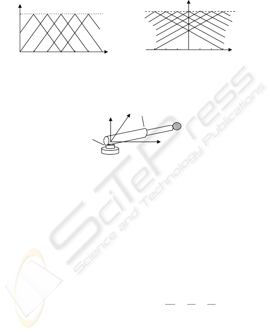
Triangular membership functions for the
performance attributes RST, OVS, OFS and for the
fuzzy tuning actions DFREQ
i
, DDAMP
i
are given
in Figure 3 and Figure 4, respectively. Each fuzzy
action or condition quantity has a representative
HIERARCHICAL MODAL CONTROL OF A NOVEL MANIPULATOR
209

value, which is assigned a membership grade equal
to unity. The decreasing membership grade around
that representative value introduces a degree of
fuzziness.
Table 4: Tuning fuzzy sets and representative numerical
values
Tuning Fuzzy Set
Notation Fuzzy Value
Integer
Value
PL Positive Large 3
PM Positive Moderate 2
PS Positive Small 1
ZR Zero 0
NS Negative Small -1
NM Negative Moderate -2
NL Negative Large -3
3 GROUND-BASED SIMULATION
3.1 Modeling of a Ground-Based
Manipulator System
The ground-based manipulator system considered
for fuzzy tuning modal control is shown in Figure 5.
The system consists of a single module manipulator
carrying a point-mass payload held by the end
effector. The module has two rigid links. The first
link undergoes slewing motion through a flexible
revolute joint. The other link can be deployed and
retrieved by the rigid prismatic joint. The motion of
the manipulator is confined to the horizontal plane,
i.e. the gravity effects are not present.
The revolute joint is considered flexible. It is
modeled by a linear torsional spring, with stiffness
K, that connects the rotor of the servomotor to the
slewing link. The angular motion of the rotor with
respect to stator is denoted by
α
. The angular
deformation of the torsional spring is given by
β
.
Thus
θ
αβ
=
+
is the total angular displacement of
the slewing link.
3.2 Control System and Simulation
Results
As mentioned before, the hierarchical structure used
combines the advantages of a crisp modal controller
with those of a soft, knowledge-based, supervisory
controller. The three layers of the structure
implement such tasks as collection of information
coming from sensors, data processing and
information abstraction, as well as general
supervisory control.
This hierarchical control system is used to
suppress the vibrations of the manipulator system
described in Figure 5. The effectiveness of the
control system is assessed by studying suppression
of vibrations caused by different disturbances. In the
first two cases, the initial disturbances at the flexible
joint of the manipulator are considered. The length
of the module may be specified at a fixed value
through the Lagrange multiplier. Therefore, the
subsystem considered for control simulation has two
Figure 2: Rulebase for the control parameter tuning.
If RST is HIUN, then DFREQ
i
is PL, DDAMP
i
is NM,
or If RST is NDIM, then DFREQ
i
is PM, DDAMP
i
is NS,
or If RST is ACCP, then DFREQ
i
is PM, DDAMP
i
is ZR,
or If RST is INSP, then DFREQ
i
is ZR, DDAMP
i
is ZR,
or If RST is OVSP, then DFREQ
i
is NS, DDAMP
i
is ZR,
or If OVS is HUIN, then DFREQ
i
is NM, DDAMP
i
is PL,
or If OVS is NDIM, then DFREQ
i
is NS, DDAMP
i
is PM,
or If OVS is ACCP, then DFREQ
i
is ZR, DDAMP
i
is PS,
or If OVS is INSP, then DFREQ
i
is ZR, DDAMP
i
is ZR,
or If OVS is OVSP, then DFREQ
i
is PS, DDAMP
i
is NS,
or If OFS is HIUN, then DFREQ
i
is PM, DDAMP
i
is NS,
or If OFS is NDIM, then DFREQ
i
is PS, DDAMP
i
is NS,
or If OFS is ACCP, then DFREQ
i
is ZR, DDAMP
i
is NS,
or If OFS is INSP, then DFREQ
i
is ZR, DDAMP
i
is ZR,
or If OFS is OVSP, then DFREQ
i
is NS, DDAMP
i
is ZR,
ICINCO 2004 - INTELLIGENT CONTROL SYSTEMS AND OPTIMIZATION
210
degrees of freedom, with
,,,
α
βαβ
&
&
as the system
state variables. The parameters for the first
simulation case are given in Figure 6.
The initial feedback control gain is determined
using the Linear Quadratic Regulator (LQR). Based
on this, tuning action takes place. The tuning process
involves analysis of the response to an initial
disturbance listed in Figure 7, with respect to the
performance requirements of rise time, overshoot,
and steady-state error. The feedback gain matrix is
updated by the supervisory controller accordingly.
Figure 7(a) shows the system response when
controlled using the LQR strategy. The initial
displacement (= 2°) of the torsional spring at the
revolute joint results in vibrations at
α
and
β
. The
suppression of the vibrations can be observed due to
the application of the LQR controller. As can be
seen, the convergence speed is slow in this case, and
significant vibration remains after 10 seconds.
Figure 7(b) shows the results after fuzzy tuning is
applied. It can be observed that the convergence
speed is much faster compared to that in the LQR
controlled case. Within 4 seconds, the vibrations in
each degree of freedom are eliminated. Further
more, the peak amplitudes of the vibrations are
sign
hnique (FLT). The desired profiles
are described as
ificantly reduced.
In the above case, the response of a ground-
based deployable manipulator, experiencing
vibrations due to the initial disturbance at the
revolute joint, was studied. To further evaluate the
effectiveness of the hierarchical control system, a
case of simultaneous 30° slew and 0.5 m deployment
in 10 seconds was considered. Now the slew motion
at the revolute joint and deployment at the prismatic
joint are controlled using the nonlinear Feedback
Linearization Tec
2
() sin
2
s
s
τπ
τ
ττ
τπτ
⎧
⎫
∆
∆
⎛⎞
=−
⎨
⎬
⎜⎟
∆∆
⎝⎠
q
q
, (11)
whe
of coo
⎩⎭
re
s
q
is the specified set rdinates ( ,l
α
);
s
∆
q
is its desired variation (
, l
α
∆∆
);
τ
is the time;
and ∆
τ
is the time required for the maneuver.
NL
NM
NS
ZR
P
S
PM
PL
0
1
2
3
-3 -2
-1
1
Figure 4: Membership functions for the fuzzy
tuning actions
Membership
Grade
Tuning
Action
1
0
2
3
4
5
1
HIUN
NDIM
ACCP
INSP
OVS
P
Figure 3: Membership functions for the fuzzy
performance attributes
Membership
Grade
Performance
Attribute
Figure 5: Configuration of the single-module manipulator with
revolute and prismatic joints
Base
x
o
Flexible Revolute
Join
t
Prismatic
Joint
Payload
y
o
z
o
HIERARCHICAL MODAL CONTROL OF A NOVEL MANIPULATOR
211

As can be expected, the large scale motions at
both revolute and prismatic joints would result in
vibration at the revolute joint, and this would persist
if damping is not present in the system. This
suggests a need for active control to suppress the
maneuver-induced vibration. To that end, two
control approaches are considered: the LQR and
Tuned Modal Control. They are applied after the
FLT- regulated maneuver is completed. Figure 8 (a)
shows the system response when controlled by the
combined FLT/LQR procedure. The rigid degrees of
freedom are regulated very well within the first 10
seconds by the FLT. After that, the LQR is applied
to suppress the maneuver-induced vibrations at the
flexible revolute joint. It is apparent that the LQR is
effective but its convergence speed is slow. Figure 8
(b) shows the system response when the
combination of the FLT and Tuned Modal Control is
employed. To obtain faster convergence speed,
tuning action is carried out based on the LQR
feedback gain matrix. It can be seen from Figure 8
(b) that, after a few tuning steps, much faster
convergence speed is achieved. The vibrations at the
flexible revolute joint are quickly eliminated right
after completion of the maneuver, without any
oscillations. Therefore, the developed knowledge-
based tuning system is quite effective in improving
the controller performance in presence of
maneuvers. It should be pointed out that, by
changing weight matrix of the LQR, a faster
response than that shown in Figure 8 (a) may be
achievable. However it is still significant to evaluate
the effectiveness of the ‘intelligent’ tuning system in
improving the controller performance.
4 CONCLUDING REMARKS
In this paper, a knowledge-based hierarchical control
system was developed for the vibration control of a
manipulator system. For this purpose, first a fuzzy
inference system (FIS) was established. The FIS was
then combined with a crisp modal controller to
construct a hierarchical control system.
The effectiveness of the hierarchical control
system was investigated through two simulation
cases. In the first case, the system was experiencing
vibration due to an initial disturbance at the revolute
joint. The second case considered a system going
through a simultaneous slew and deployment
maneuver. The results showed that the knowledge-
based tuning system developed here was quite
effective. It was found that the performance of a
modal controller for a manipulator could be
significantly improved through knowledge-based
tuning. On this basis one might conclude that
additional tuning of the controller parameters could
significantly improve the performance of a modal
controller in general.
System Parameters
Slewing link:
= 1.0 m
1
l
= 2.0 kg
1
m
Deployable link:
= 1.0 m
2
l
= 2.0 kg
2
m
Payload:
= 3.0 kg
p
m
Joint stiffness:
K = 80 Nm/rad
Rotor inertia:
J = 2 kg-
2
m
Specified Coordinates
l = 1.5 m
(i.e., length is held fixed.)
Initial Conditions
(0) 0
α
= , ; (0) 2
β
=
o
(0) (0) 0.
αβ
==
&
&
α
β
o
x
o
y
l
Figure 6: Parameters for the ground-based simulation.
ICINCO 2004 - INTELLIGENT CONTROL SYSTEMS AND OPTIMIZATION
212
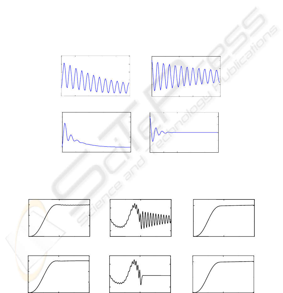
Figure 7: System response to an initial displacement at the revolute joint:
(a) controlled by LQR; (b) controlled by hierarchical controller.
2
68
Time, s
0 2
4
6
8 10
-2
-1
0
1
2
β
o
0 2 4 6 8 10
-1
0
1
2
3
4
α
o
(a)
2 4 6
Time, s
0
4
10
-2
-1
0
1
2
β
o
0 8
10
0
1
2
3
α
o
(
b
)
ACKNOWLEDGEMENT
Funding for the work reported in this paper has
come from the Natural Sciences and Engineering
Research Council of Canada.
REFERENCES
Junkins, J.L., 1993. Introduction to Dynamics and
Control of Flexible Structures, American Institute of
Aeronautics and Astronautics, Inc., Washington,
DC, U.S.A., pp. 235-265.
Nishitani, A., 1998. Application of Active Structural
Control in Japan, Progress in Structural Engineering
and Materials, Vol. 3, pp. 301-307.
de Silva, C. W., 1995. Intelligent Control: Fuzzy Logic
Applications, CRC Press, Boca Raton, FL, U.S.A.
Goulet, J. F., 1999. Intelligent Hierarchical Control of a
Deployable Manipulator, M.A.Sc. Thesis,
Department of Mechanical Engineering, University
of British Columbia. Vancouver, B.C.
de Silva, C.W., 2000. Vibration Fundamentals and
Practice, CRC Press, Boca Raton, FL, U.S.A.
Caron, M., Modi, V. J., Pradhan, S., de Silva, C. W., and
Misra, A.K., 1998. Planar Dynamics of Flexible
Manipulators with Sewing and Deployable Links,
Journal of Guidance, Control, and Dynamics, Vol.
24, pp. 572-580.
01
2
Time, s
Time, s
Time, s
0
1
2
3
α
o
-
0.2
0
0.
β
o
1
1.
l, m
(a)
(b)
Figure 8: System response while going through a maneuver:
(a) controlled by the FLT/LQR;
(b) controlled by the FLT/Tuned Modal Control.
0
1
2
3
α
o
-
0.2
0
0.
β
o
1
1.
l, m
01
2
01
2
01
2
01
2
01
2
HIERARCHICAL MODAL CONTROL OF A NOVEL MANIPULATOR
213
