MOTION PLANNING FOR MOBILE ROBOTS IN DYNAMIC
ENVIRONMENTS
Jing Ren, Kenneth.A. McIsaac and Xishi Huang
University of Western Ontario
London ON, Canada N6G 1H1
Keywords:
Potential field, multi-robot motion planning, stability, dynamic environment.
Abstract:
In this paper, we present a motion planning technique for a multi-robot team in a complex dynamic environ-
ment. We define a cell-based navigation control law that can guide the robot team through the environment
while avoiding collisions with both static and dynamic obstacles and other team members. To illustrate our
techniques, we consider a robot team motion planning problem in a complex “maze” with obstacles of arbi-
trary shape. First, we assign potential values to a set of landmarks based on their shortest distance to the goal,
and then we use a spline function to generate a potential field for the entire workspace, which is inherently
free of undesired local minima. Simulation results show that robots can successfully transport materials along
an optimal and collision-free path and reach the goal in a complex and dynamic maze environment. Finally
we prove the derived control law is stable in all times.
1 INTRODUCTION
A central issue in mobile robotics is navigation strat-
egy. Potential field approaches are widely used for
motion planning in mobile robotics because of their
simplicity and elegance. In Koditschek’s basic for-
mulation (Koditschek 1989), a scalar field compris-
ing artificial “hills” (representing obstacles, or other
robots) and “valleys” (attractive positions) in the
robot’s world map lead naturally to a stable path to-
wards a “low-energy” goal position. Extensive work
has been done for single robot navigation. But much
less investigation is devoted to a team navigation in
the dynamic and complex environment.
Although single robots can play an important role
in many areas, the use of multi-robot teams has a
number of potential advantages over single robot sys-
tems. A group of robots working together can accom-
plish the task of a complex, purpose-built system in
a fraction of the time, and the built-in redundancy of
having many team members leads to a more robust-
ness and fault tolerance.
Dynamic environment is a recurring challenge in
motion planning. Robots providing services in sewer
systems, office buildings, supermarkets or even pri-
vate homes must be able to adapt on-line to un-
predictable dynamic obstacles, such as people going
about their own business. For a single robot, Espos-
ito (Esposito 2002) proposed a technique to treat un-
predictable obstacles as dynamic constraints that limit
the choices of feasible trajectories. In this paper, we
modified and extended this technique to a robot team.
2 PROBLEM STATEMENT
We consider a team of robots operating in a complex
and dynamic maze environment that is populated with
static obstacles of arbitrary geometry and a number
of unpredictable moving obstacles. The configuration
q
i
of each robot is given by the vector q
i
=(x
i
,y
i
)
of the position of its center of mass. We also define
q =(q
1
,q
2
, ..., q
Q
) as the state vector of the robot
team, Q is the number of the robots.
The robots task is to transport materials in a maze,
tracking the shortest path from any starting point to
a defined goal position and avoiding collision with
the environment (fixed obstacles); with their team
members, and with a set of randomly moving, unpre-
dictable dynamic obstacles.
361
Ren J., A. McIsaac K. and Huang X. (2004).
MOTION PLANNING FOR MOBILE ROBOTS IN DYNAMIC ENVIRONMENTS.
In Proceedings of the First International Conference on Informatics in Control, Automation and Robotics, pages 361-364
DOI: 10.5220/0001128503610364
Copyright
c
 SciTePress

3 POTENTIAL FIELD
CONSTRUCTION
Our idea of potential field construction is based on
the shortest distance transform. The potential values
of a set of known landmarks are first defined accord-
ing to their shortest distance to the goal. Then we
use a spline function based on these known poten-
tial values to generate a potential field for the en-
tire workspace. Along with this shortest-distance-
based potential field, our navigation function includes
avoidance of known dynamic obstacles (other robots
in the team, modelled by a generalized Gaussian func-
tion). Unknown dynamic obstacles are treated as run-
time constraints on the motion plan that are only acti-
vated when obstacles are detected “near” the navigat-
ing robot.
3.1 Distance Transform
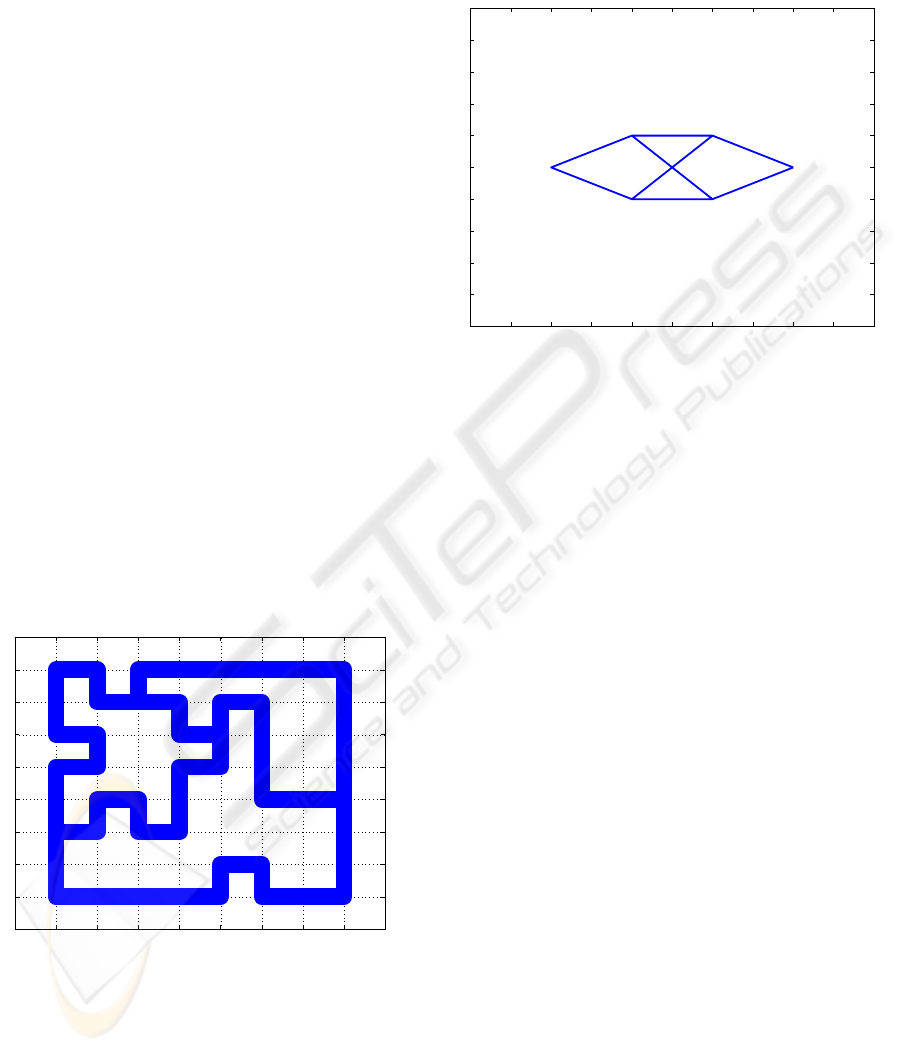
The simple example maze in Figure 1 illustrates our
technique of using landmarks to map the workspace
into a node network based on the distance transform.
In the figure, the dark lines represent feasible paths
through the maze from point A to point D. Points B1,
B2, C1 and C2 are considered waypoints, which es-
sentially represent “forks” where the planning algo-
rithm will have to make choices. In our present work,
the task of generating these waypoints is left to the
programmer, although we believe it will be a simple
matter to automate this step.
0 1 2 3 4 5 6 7 8 9
0
1
2
3
4
5
6
7
8
9
A
O
O
O
O
O
O
B1
B2
C2
C1
D
Figure 1: The original map of a simple maze. A is the start-
ing point, and D is the goal point. B1, B2, C1 and C2 are
all waypoints, where the planner must make a decision.
After finding the required set of landmarks, we can
generate a node network. The equivalent network for
the maze of Figure 1 is given in Figure 2. In this
graph, one node is associated with each landmark, and
the values of edges connecting nodes are given by the
distance between landmarks. Since there are no forks
between pairs of landmarks, there is a non-ambiguous
value for each of these edges.
0 1 2 3 4 5 6 7 8 9 1
0
0
1
2
3
4
5
6
7
8
9
1
0
O
O
O
O
O
O
Goal
Start
3
6
4
7
2
7
10
14
A(16)
B1(9)
B2(16)
C1(6)
C2(4)
D(0)
Figure 2: Node network corresponding to the workspace of
Figure 1. The numbers in parentheses represent the short-
est distance (potential value) of each node to the goal. The
numbers on the edges represent the distance between the
associated pairs of nodes.
Remark: With this model of the environment, there
are various methods to find the optimal path through a
graph for different applications. In our simulation, we
use the techniques of dynamic programming to gen-
erate optimal path.
3.2 Construction of the Potential
Field Model
In this section, we will discuss how we develop a po-
tential field model of the workspace that incorporates
both obstacles and robots.
We define a bicubic spline over the workspace. The
potential values of landmarks are the shortest dis-
tances to the goal. Potential values at cell corner
points that fall inside feasible regions are also the
shortest distances to the goal, which is the addition
of the potential values of the landmarks and the dis-
tance to those landmarks. Potential values at cell cor-
ner points that fall inside obstacles can be defined es-
sentially arbitrarily, provided they are given a larger
value than that of neighboring cell corners in feasible
region.
Given any position q =(x, y) in the workspace,
the bicubic spline defines a potential field VS (q) in
cell (i, j) of the form
VS (q)=S
i,j
(x, y)=
3

k=0
3

l=0
a
(i,j)
k,l
(x−x
i
)
k
(y−y
j
)
l
(1)
ICINCO 2004 - ROBOTICS AND AUTOMATION
362

where (x
i
,y
j
) is the position of left bottom corner
point of cell (i, j), a
(i,j)
k,l
’s are constants determined
by the potential values of all the cell corners in the
entire workspace. According to the spline theory,
VS (q) has continuous second derivative in the entire
workspace.
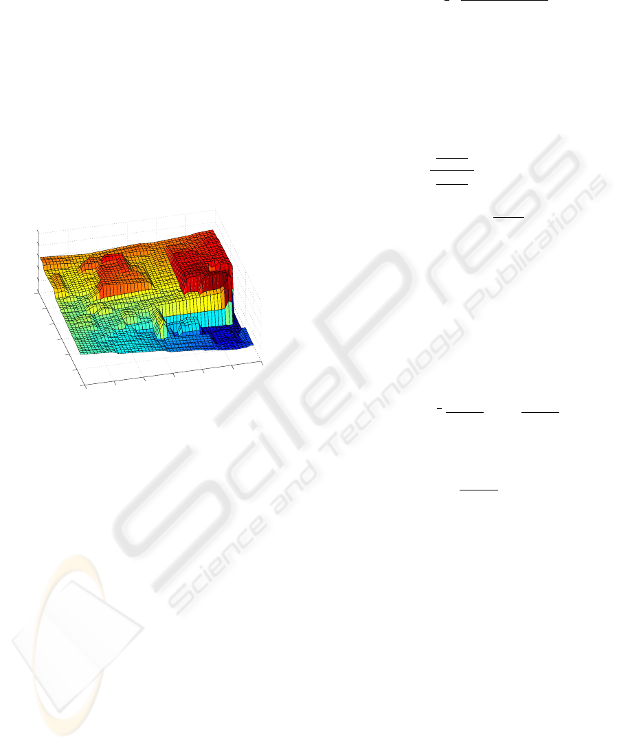
The potential field thus created gives a smooth ap-
proximation of the optimal distance from each point
in the maze to the goal. Note that although we include
a “start” point in our dynamic programming analy-
sis, our interpolating spline function gives the optimal
path from any arbitrary starting point anywhere in the
maze. Figure 3 shows the potential field for an exam-
ple maze.
0
5
10
15
20
25
30
0
5
10
15
20
25
30
0
100
200
300
400
500
Figure 3: Potential field of an example maze. The lowest
point is the goal. The potential values of points in the maze
depend both on their type (obstacle or path) and also on the
shortest distance to the goal. Although the user must only
distinguish obstacles from safe points, we can see clearly
from this plot that points of the same type take on smaller
and smaller potential values as they get closer and closer to
the goal.
4 MOTION PLANNING
4.1 Navigation Function
To construct the navigation function for each robot
we use the two part formula:
V
i
(q)=VS (q
i
)+
j⊆G
i

j=i
VR (q
i
,q
j
) (2)
where G
i
is defined as the set of team members within
the protective space of agent i, VS (q
i
) represents the
optimal potential field generated by our interpolating
cubic spline, and the functions VR (q
i
,q
j
) represent
the repulsor functions between pairs of robots i and j.
VR (q
i
,q
j
)=e
−
1
2

(x
i
−x
j
)
2
+(y
i
−y
j
)
2
σ
2

C
(3)
using the generalized Gaussian repulsor function.
4.2 Control Law without Moving
Obstacles
For every system state, q, we associate with each
robot, i, a control law, u
i
(q), of the form:
u
i
(q)=−α
∂V
i
(q)
∂q
i



∂V
i
(q)
∂q
i



,i=1, 2, ..., Q (4)
In Equation 4.2, the operator
∂V
i
(q)
∂q
i
represents the
gradient of V
i
(q) with respect to only q
i
.
4.3 Control Law with Moving
Obstacles
For every system state, q, we associate with each
robot, i,afeasible control generating function,to
move the robot away from nearby unmodelled obsta-
cles while still making progress to the goal, Z
i
(q),of
the form:
Z
i
(q)=−(1 − β
2
)
1
2
∂V
i
(q)
∂q
i
+ β

∂V
i
(q)
∂q
i

⊥
(5)
provided β
2
< 1. With this definition for Z
i
(q),we
define the control law for the robots as:
˙q
i
= α
Z
i
(q)
|Z
i
(q)|
(6)
In this control law, the feasible control function,
Z
i
(q), generates a unit vector direction for the robot,
and the constant velocity parameter α is used to
choose the robot’s speed.
5 STABILITY ANALYSIS
We can define a Lyapunov function for the team of the
form:
V
X
(q)=
Q

i=1
V
X
i
i
(q) −
Q

i=1
j⊆G
i

j≥i+1
VR (q
i
,q
j
)(7)
=
Q

i=1
VS (q
i
)+
Q

i=1
j⊆G
i

j≥i+1
VR (q
i
,q
j
)(8)
where the step from Equation 7 to Equation 8 is
justified by the fact that VR (q
i
,q
j
)=VR (q
j
,q
i
).
MOTION PLANNING FOR MOBILE ROBOTS IN DYNAMIC ENVIRONMENTS
363

To show Lyapunov stability, we are required to show
V (q) ≥ 0 ∀q and
˙
V (q) < 0 ∀q, t. In Equation 8, the
first term represents the potential value at the robot
position, which is defined as the shortest distance to
the goal and therefore is positive by construction; Ac-
tually the first part is the potential field of workspace
generated from the bicubic spline function. Due to
the features of our problem, we are only concerned
about the relative potential difference of the positions
in the workspace but not the absolute potential value
of each position. Therefore in the implementation we
can always add an arbitrary positive potential value
to all positions and guarantee this part is positive.
That the second term is also positive follows naturally
from the definition of VR(q
i
,q
j
), As a result, we have
V (q) ≥ 0 by construction.
To show that V (q) is always decreasing, we begin us-
ing the form of Equation 7. For convenience, in the
derivations that follow, we have replaced terms of the
form VR (q
i
,q
j
) with the short form VR
ij
:
Thus, the second and third terms will cancel(Ren
2003), and we will have:
˙
V (q)=
Q

i=1

∂V
i
(q)
∂q
i

T
˙q
i
(9)
If we substitute for ˙q
i
using the dynamics defined in
Section 4.2, we will have:
˙
V (q)=−
α
|Z
i
(q)|
Q

i=1
(1 − β
2
)
1
2

∂V
i
(q)
∂q
i

T
∂V
i
(q)
∂q
i
−
α
|Z
i
(q)|
Q

i=1
β

∂V
i
(q)
∂q
i

T

∂V
i
(q)
∂q
i

⊥
(10)
= −
α
|Z
i
(q)|
Q

i=1
(1 − β
2
)
1
2

∂V
i
(q)
∂q
i

T
∂V
i
(q)
∂q
i
Because β
2
< 1, we will have
˙
V (q) < 0 ∀t, q as
required.
6 SIMULATION RESULTS
In simulation, we use dynamic programming to find
the shortest path to the goal from a set of known way-
points where decisions will need to be made by a path
planner and the construction of a potential field based
on a bicubic spline function that generates the shortest
path from all points in the map with C
2
continuity.
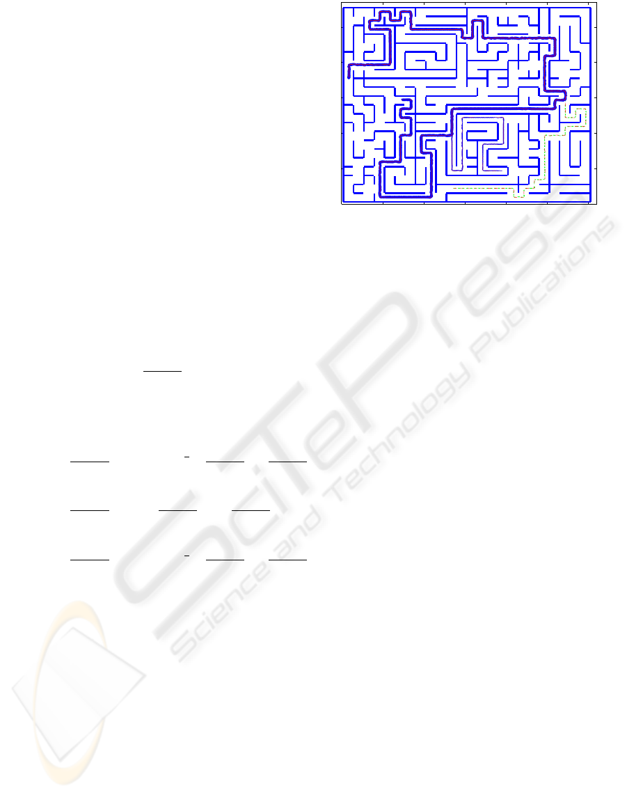
In Figure 4, we show the results from a sample sim-
ulation of a three-robot team transporting materials in
a maze. All three robots find the shortest path from
their start positions to the goal, and travel the short-
est path while avoiding collisions with obstacles and
their fellows.
0 5 10 15 20 25 30
0
5
1
0
1
5
2
0
2
5
R1
R2
R3
GOAL
Figure 4: R1,R2,R3 are 3 robots. The different line styles
represent trajectories of different robots. The three robots
start in different initial positions, and all find the optimal
(shortest) path to the goal, while avoiding collisions with
each other.
7 CONCLUSIONS AND FUTURE
WORK
In this paper, we present a technique for an agent-
based multi-robot team finding the optimal path
through a complex maze in the presence of dynamic
obstacles. By modifying and extending Esposito’s
moving strategy to a robot team, we define a control
law that incorporates moving obstacles avoidance.
REFERENCES
Esposito J.M. and Kumar, V. A method for modify-
ing closed-loop motion plans to satisfy unpredictable
dynamic constraints at run-time. In Proc. IEEE
Int. Conf. Robotics and Automation, pages 1691–
1696, Washington, May 2002.
Koditschek, D.E. Robot planning and control via potential
functions. In O. Khatib, J. J. Craig, and T. Lozano-
Perez, editors, The Robotics Review 1, pages 349–367,
1989.
J. Ren, K. A. McIsaac. A Hybrid Systems Approach to
Potential Field Navigation for a Multi-Robot Team. In
Proc. IEEE Int. Conf. Robotics and Automation, pages
3875–3880, Taipei, Sept 2003.
ICINCO 2004 - ROBOTICS AND AUTOMATION
364