
PARAMETER CONVERGENCE IN ADAPTIVE FUZZY CONTROL
Domenico Bellomo, David Naso
Dipartimento di Elettronica ed Elettrotecnica, Politecnico di Bari
Via Re David 200, 70125 Bari, Italy
Robert Babu
ˇ
ska
Delft Center for Systems and Control, Delft University of Technology
Mekelweg 2, 2628 CD Delft, the Netherlands
Keywords:
Adaptive fuzzy control, tracking control, identification, feedback linearization, interactions.
Abstract:
In this paper, the convergence of parameter estimates and the interactions among the two adaptive fuzzy
systems constituting an indirect adaptive fuzzy controller are studied, both analytically and by means of sim-
ulations with a second-order nonlinear system. The analytical results and the simulations, performed with
various initial conditions and learning rates, highlight how the interactions affect the behavior of the adaptive
control scheme with regard to the control performance in terms of a tracking error, accuracy and relevance of
the identified fuzzy models.
1 INTRODUCTION
The main goals of adaptive control are (i) to adjust
the on-line controller such that the required closed-
loop performance (stability in the first place) is pre-
served in the presence of unforeseen parameter vari-
ations and/or (ii) to learn a suitable control law when
a priori information on the controlled plant is lacking
(e.g., theplant parameters are partly or completely un-
known).
Adaptive fuzzy control (AFC) combines results
from modern control theory, fuzzy systems and adap-
tation techniques. The most common stable AFC
schemes are based on feedback linearization, employ-
ing fuzzy systems (mostly of the singleton type) as
universal function approximators. They can be used
either to approximate the unknown plant dynamics
(indirect schemes) or directly the control law (direct
schemes). With respect to other universal interpola-
tors, such as neural networks, fuzzy systems offer the
possibility to interpret the input-output relations by
means of linguistic rules. This feature allows one to
incorporate a priori knowledge in the initial model
and/or control law and, at least in principle, to gather
useful insights about the controlled process at the end
of the learning stage.
The parameter learning laws of AFC are often de-
rived by using Lyapunov synthesis (Wang, 1994) and
are basically guided by the tracking error with respect
to some reference trajectory. The earliest controllers
of this type have been introduced for SISO systems in
the controllable canonical form (Wang, 1993; Wang,
1996). Since then, considerable efforts have been de-
voted to improving the performance and extending
the applicability to wider classes of systems. For
instance, extensions to systems with unmeasurable
states are proposed in (Tong et al., 2000), MIMO sys-
tems are considered in (Ordonez and Passino, 1999;
Tong and Chai, 1999), while in (Wang et al., 2002;
Tsay et al., 1999; Spooner and Passino, 1996) first-
order Takagi-Sugeno fuzzy systems are used as ap-
proximators. Adaptive fuzzy control in the presence
of uncertainties is realized by adding a sliding mode
term to the control law (Su and Stepanenko, 1994;
Han et al., 2001; Fishle and Schroder, 1999), or by
using H
∞
performance indices (Chen et al., 1996;
S. Tong and Wang, 2000).
Despite numerous studies on AFC, some basic
problems arising even in the case of simple nonlinear
SISO systems have not been addressed in the litera-
ture. Examples of these problems are:
• dependence of the AFC performance (learning
time, stability of the adapted parameters and qual-
ity of the identified models) on user-defined param-
eters;
• inherent conflict between the control goal (reduc-
tion of the tracking error) and the identification
goal (reduction of the identification error with re-
spect to the unknown system dynamics);
135
Bellomo D., Naso D. and Babuška R. (2004).
PARAMETER CONVERGENCE IN ADAPTIVE FUZZY CONTROL.
In Proceedings of the First International Conference on Informatics in Control, Automation and Robotics, pages 135-142
DOI: 10.5220/0001128701350142
Copyright
c
SciTePress

• interactions between the fuzzy systems’ parame-
ters and their convergence during the learning pro-
cess.
The lack of a proper understanding of these basic as-
pects makes it difficult to properly exploit the trans-
parency and interpretability of fuzzy systems, which
are in fact neglected in a considerable part of the re-
cent literature on AFC.
In this paper, we address the issue of interaction
between the fuzzy systems’ parameters and their con-
vergence in the case of indirect AFC based on feed-
back linearization. First, we determine analytical re-
lations between the rates of change of the tracking er-
ror and the parameter errors. This analysis highlights
the occurrence of conflicts between the identification
of unknown system dynamics and the tracking con-
trol. Then, we show, by means of simulations with a
second-order system, that the AFC performance criti-
cally depends on user-defined parameters such as the
learning rates or initial values of the adapted parame-
ters. We consider the scheduling of learning rates as
a possible solution to overcome the above-mentioned
problems.
The remainder of this paper is structured as fol-
lows. In Section 2, the basic elements of indirect
adaptive fuzzy control are described. In Section 3,
an analysis of interactions is carried out. Section 4
describes a case-study with a second-order nonlinear
system. The scheduling of the learning rates and its
effects on the performance are discussed in Section 5.
Finally, in Section 6, conclusions are given.
2 INDIRECT AFC
2.1 Structure of the Controller
Indirect adaptive fuzzy control (Wang, 1996) is suit-
able for systems in controllable canonical form
x
(n)
= f(x)+g(x)u (1)
y = x. (2)
where x =
x, ˙x,...,x
(n−1)
T
∈ R
n
is the state
vector. The control goal is to track a desired trajec-
tory y
m
while keeping all the signals bounded in the
closed-loop. Define the tracking error e = y
m
− y
as the difference between the reference trajectory and
the output of the system. Further, introduce the vec-
tor of the tracking error and its n − 1 derivatives
e =
e, ˙e,...,e
(n−1)
T
and the vector of the feed-
back gains k =[k
n
,...,k
1
]
T
. If the functions f(x)
and g(x) are known and if the gains k
i
are cho-
sen such that the roots of the polynomial h(s)=
s
n
+ k
1
s
n−1
+ ...+ k
n
are in the open left-half com-
plex plane, the feedback linearizing control law
u
∗
=
1
g(x)
−f(x)+y
(n)
m
+ k
T
e
(3)
produces the desired linear error dynamic:
e
(n)
+ k
T
e =0 (4)
or equivalently
˙
e = Λ
c
e (5)
where the matrix Λ
c
∈ R
nxn
is given by
Λ
c
=
⎡
⎢
⎢
⎢
⎢
⎢
⎣
010... 0
001
.
.
.
.
.
.
.
.
.
.
.
.
.
.
.
.
.
.
0
00... 01
−k
n
−k
n−1
... ... −k
1
⎤
⎥
⎥
⎥
⎥
⎥
⎦
. (6)
The ideal control law (3) guarantees that
lim
t→∞
e(t)=0. The basic idea of Wang’s
indirect adaptive control is to approximate the
unknown functions f(x) and g(x) in the control law
(3) by using two singleton fuzzy systems:
ˆ
f(x)=θ
T
f
ξ
f
(x) (7)
ˆg(x)=θ
T
g
ξ
g
(x) . (8)
where θ
f
and θ
g
are the consequent parameters to be
adapted, ξ
f
(x) and ξ
g
(x) are the normalized degrees
of fulfillment of the (fixed) fuzzy rules. If we replace
the functions f (x) and g(x) in (3) with their fuzzy
approximations, we have a control law
u =
1
ˆg(x)
−
ˆ
f(x)+y
(n)
m
+ k
T
e
(9)
that is an approximation of the ideal law (3). To
properly isolate the effects of interactions between
the learning systems from other phenomena related
to the minimal approximation error, we choose f(x)
and g(x) that can be exactly approximated by the two
fuzzy systems
ˆ
f(x) and ˆg(x): f (x)=θ
∗
f
T
ξ(x) and
g(x)=θ
∗
g
T
ξ(x) (where θ
∗
f
and θ
∗
g
represent the op-
timal parameters). Adding and subtracting ˆg(x)u at
the right-hand side of (1), substituting the control law
(9) only in the term ˆg(x)u and substituting equations
(7), (8) with the actual and optimal parameters, we
have, after some manipulations, the error dynamic
˙
e = Λ
c
e + b
c
φ
T
f
ξ
f
(x)+φ
T
g
ξ
g
(x)u
(10)
where b
c
=[0, ..., 0, 1]
T
; the parameter error φ
f
=
θ
f
− θ
∗
f
is the difference between the actual param-
eters θ
f
of the fuzzy system
ˆ
f(x) and the optimal
parameters θ
∗
f
; the same holds for the parameter error
φ
g
= θ
g
− θ
∗
g
.
ICINCO 2004 - INTELLIGENT CONTROL SYSTEMS AND OPTIMIZATION
136

2.2 Adaptive Laws
The adaptive laws are derived using Lyapunov syn-
thesis. The considered Lyapunov function
V =
1
2
e
T
Pe +
1
2γ
f
φ
T
f
φ
f
+
1
2γ
g
φ
T
g
φ
g
= V
e
+ V
f
+ V
g
. (11)
is the sum of three contributions depending respec-
tively on the tracking error e and the parameter errors
φ
f
and φ
g
. Matrices P ∈ R
nxn
and Q ∈ R
nxn
are positive-definite matrices that fulfill the Lyapunov
equation
Λ
T
c
P + PΛ
c
= −Q . (12)
This choice for V is made with the goal of guaran-
teeing simultaneously the boundedness of tracking er-
ror and of parameter errors. The time-derivative of V
is obtained by differentiating (11), substituting for
˙
e
from (10) and using (12)
˙
V = −
1
2
e
T
Qe +
1
γ
f
φ
T
f
˙
θ
f
+ γ
f
e
s
ξ
f
(x)
+
1
γ
g
φ
T
g
˙
θ
g
+ γ
g
e
s
ξ
g
(x) u
(13)
where γ
f
and γ
g
are the learning rates, e
s
= e
T
p
n
and p
n
is the last column of P. If the parameters θ
f
and θ
g
are adapted according to the following laws
˙
θ
f
= −γ
f
e
s
ξ
f
(x) (14)
˙
θ
g
= −γ
g
e
s
ξ
g
(x) u (15)
the terms in the brackets in (13) are zero and the
derivative
˙
V is negative-definite. This guarantees that
V is decreasing and asymptotically converges to zero.
3 ANALYSIS OF INTERACTIONS
This section focuses on the interactions between the
two adaptive fuzzy systems (7) and (8) and the effects
of these interactions on the evolution of the tracking
error and the parameter errors. In (13) we can separate
the time derivatives of the terms V
f
, V
g
and V
e
:
˙
V
f
=
1
γ
f
φ
T
f
˙
θ
f
(16)
˙
V
g
=
1
γ
g
φ
T
g
˙
θ
g
(17)
˙
V
e
= −
1
2
e
T
Qe + e
s
φ
T
f
ξ
f
(x)+e
s
φ
T
g
ξ
g
(x)u (18)
If we substitute the expression of
˙
θ
f
given by (14) in
(16), remembering the definition of φ
f
we get
˙
V
f
= −e
s
φ
T
f
ξ
f
(x)=−e
s
ˆ
f(x) − f (x)
. (19)
In the same way, substituting
˙
θ
g
from (15) into (17)
and recalling the definition of φ
g
, we obtain
˙
V
g
= −e
s
φ
T
g
ξ
g
(x)u = −e
s
(ˆg(x) − g(x)) u. (20)
Substituting the control law (9) into ˆg(x)u and deriv-
ing from (1) the product g(x)u, we can recast the last
equation in the following form (after some manipula-
tions):
˙
V
g
= −
˙
V
f
− e
s
e
(n)
+ k
T
e
. (21)
In the same way, we can prove that
˙
V
e
= −
1
2
e
T
Qe + e
s
e
(n)
+ k
T
e
. (22)
Equations (19), (21) and (22) represent the contribu-
tions to
˙
V due to the parameter errors and the tracking
error, respectively. They highlight how the adaptive
systems interact and how such interactions affect the
identification task (reduction of the parameter errors)
and the control task (reduction of the tracking error).
The term in square brackets in equations (21) and (22)
represents the error dynamic if the control law is the
ideal feedback linearizing control law u
∗
. Hence, in
the ideal case, it is zero. Since we only have an ap-
proximation of this ideal control law, this term is not
zero. However, we can expect that if the approxi-
mation of the ideal control law is good enough, the
error will approximatively fulfill the ideal error dy-
namic and the term in square brackets will be small
compared to −
˙
V
f
(see the simulations results in Sec-
tion 4). As a result, we can see from equations (19)
and (21) that, the variations of V
f
and V
g
would be
of opposite sign: an improvement in the identification
of f(x) would be compensated by a deterioration in
the identification of g(x) and vice-versa. Equation
(22), on the other hand, shows the interference be-
tween identification and control tasks.
Remark: Note that we have not considered an ap-
proximation error. In the presence of a minimal ap-
proximation error, an additional term appears in the
time-derivative of the Lyapunov equation, but the re-
lationship between
˙
V
f
and
˙
V
g
remains unchanged.
4 SIMULATION EXAMPLE
Consider the following second-order nonlinear sys-
tem:
˙x
1
= x
2
(23)
˙x
2
= −x
2
+ g(x
1
) u (24)
y = x
1
. (25)
The functions f(x
2
)=−x
2
and g(x
1
) are chosen
such that they can be exactly represented by fuzzy
PARAMETER CONVERGENCE IN ADAPTIVE FUZZY CONTROL
137
−1.5 −1 −0.5 0 0.5 1 1
.5
−1.5
−1
−0.5
0
0.5
1
1.5
x
2
f(x
2
)
(a) Final approximation for f(x
2
)
0 1 2 3 4 5
6
0
10
20
30
40
x
1
g(x
1
)
(b) Final approximation for g(x
1
)
Figure 1: Final approximations for f (x
2
) and g(x
1
): ’o’
represent the true parameters; ’*’ represent the actual pa-
rameters.
systems with a finite number of rules. This means
that there is no minimal approximation error. In fact,
f(x
2
) is linear and g(x
1
) is a singleton fuzzy sys-
tem (with four singleton consequents and four an-
tecedent triangular membership functions centered at
x
1
=0, 2, 4, 6). The consequents are the values of
the parabolic function x
1
2
+1 for x
1
=0, 2, 4, 6. The
fuzzy system ˆg(x
1
) has the same structure as g(x
1
)
and hence it can exactly approximate g(x
1
). Another
distinct feature of the above system is that f(x) and
g(x) only depend on one component of the state vec-
tor each. This makes it possible to study the inter-
actions between adaptive fuzzy systems by using two
simple fuzzy systems with one premise variable.
The simulations have been performed with
the Matlab/Simulink implementation of the ode45
Dormand-Prince method and the relative tolerance of
0.001. Thanks to the absence of inherent approxi-
mation error in our case-study, supervisory control
is not necessary for stability assurance and is there-
fore omitted. The fuzzy systems
ˆ
f(x
2
) and ˆg(x
1
)
have four triangular membership functions equally
distributed in their respective domains, [−1.5, 1.5]
and [0, 6]. The reference model is a second order
linear system with natural frequency ω
n
=1rads
−1
and damping ratio δ =0.9. The reference signal r
m
is represented by a repeating sequence with values in
the range [0, 6].
The feedback gains k
i
were set to k
1
=1.8 and
k
2
=1. The positive-definite symmetric matrices P
and Q satisfying equation (12) were obtained by nu-
merically solving this linear matrix inequality (LMI).
4.1 Standard Setting
An attempt to train
ˆ
f(x
2
) and ˆg(x
1
) simultaneously
(with equal learning rates γ
f
= γ
g
= 100) results
in poor approximations of the true functions f(x
2
)
and g(x
1
), see Fig. 1. This is despite the fact that an
important piece of prior knowledge was used, namely
the fact that each of the functions only depends on one
component of the state.
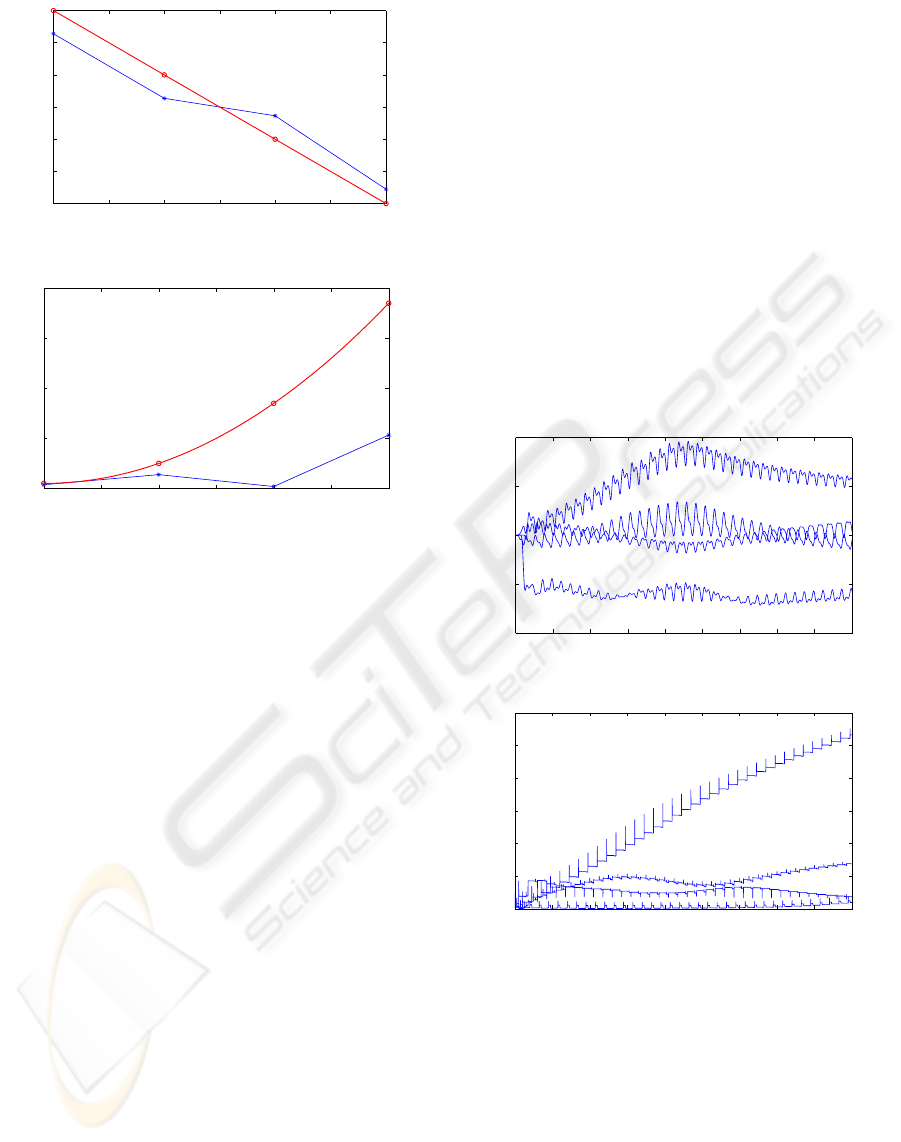
It can also be seen in Fig. 2 that in this case the
parameters are not converging at all. The analysis of
0 200 400 600 800 1000 1200 1400 1600 180
0
−2
−1
0
1
2
t [s]
θ
f
(a) Filtered singletons for f(x
2
)
0 200 400 600 800 1000 1200 1400 1600 1800
0
2
4
6
8
10
12
t [s]
θ
g
(b) Singletons for g(x
1
)
Figure 2: Singletons for f(x
2
) and g(x
1
).
interactions carried out in Section 3 offers an expla-
nation of this simulation results. In Fig. 3, we can
see that γ
f
V
f
and γ
g
V
g
exhibit similar complemen-
tary variations (the interplay between the two iden-
tification tasks): if γ
f
V
f
decreases, γ
g
V
g
increases
and vice-versa. The simultaneous identification of the
unknown system dynamics cannot be accomplished
most of the time. Moreover, in Fig. 4 we can see
the interplay between identification and control: an
improvement in the parameter errors corresponds to
ICINCO 2004 - INTELLIGENT CONTROL SYSTEMS AND OPTIMIZATION
138
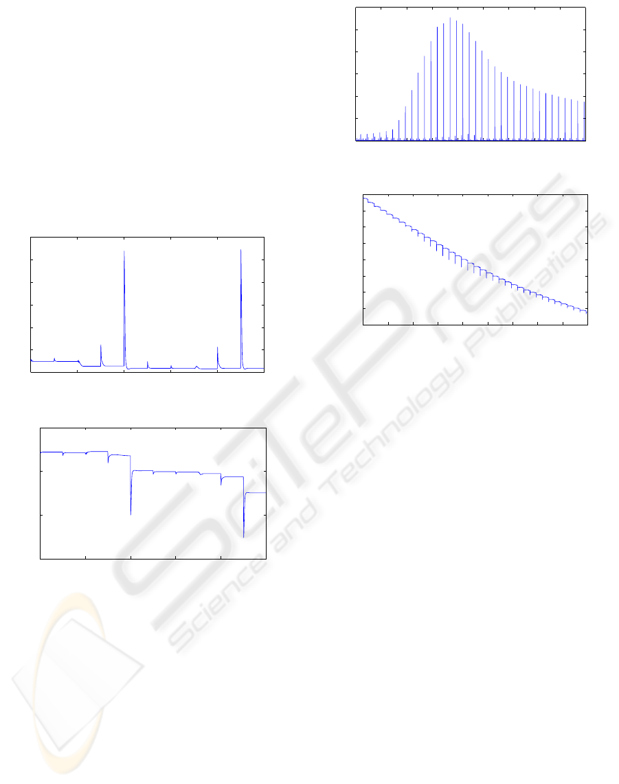
higher tracking error and vice-versa. Hence, we can
see that the adaptation is negatively affected by these
interactions, in terms of learning time, oscillation of
the parameters and accuracy of the final fuzzy models.
Remark 1: For sake of clear presentation, the pa-
rameters shown in Fig. 2(a) were filtered by a low-
pass Butterworth filter with the cut-off frequency of
0.3 rad s
−1
. Without this filtering, the plot is rather
confusing due to large overlapping parameter oscilla-
tions.
Remark 2: We have plotted γ
f
V
f
and γ
g
V
g
rather
than V
f
and V
g
because we are interested in the evolu-
tion over time of the parameter errors and the learning
rates represent just scaling factors.
0 20 40 60 80 10
0
0
10
20
30
40
50
60
t [s]
γ
f
Vf
(a) γ
f
V
f
0 20 40 60 80 10
0
1550
1600
1650
1700
t [s]
γ
g
Vg
(b) γ
g
V
g
Figure 3: Zoom on the evolution over time of γ
f
V
f
and
γ
g
V
g
.
4.2 Alternative Settings
The simulations have been also carried out in differ-
ent settings, in order to see how the phenomena high-
lighted in the previous section depend on the particu-
lar settings and to what extent they can be generalized.
First, one of the two functions f(x
2
) and g(x
1
) is
assumed to be known and the other one is learnt. This
allows us to study what happens when there are no
interactions between the learning processes. Second,
f(x
2
) and g(x
1
) are learnt simultaneously, but in this
case with different learning rates and with different
0 200 400 600 800 1000 1200 1400 1600 180
0
0
0.05
0.1
0.15
0.2
0.25
t [s]
Ve
(a) V
e
0 200 400 600 800 1000 1200 1400 1600 180
0
900
1000
1100
1200
1300
1400
1500
1600
1700
t [s]
γ
f
Vf+ γ
g
Vg
(b) γ
f
V
f
+ γ
g
V
g
Figure 4: Evolution over time of V
e
and γ
f
V
f
+ γ
g
V
g
.
initial conditions for their parameters. Finally, simu-
lations have been carried out in which the two fuzzy
systems have both states as premise variables (less
prior knowledge on the system structure is used).
4.2.1 Separate Adaptation of
ˆ
f(x
2
) and ˆg(x
1
)
First, we adapt only f (x
2
), assuming that g(x
1
) is
known. The learning rate is γ
f
= 100. At the
end of the learning, after 1800s, we get a good ap-
proximation of f (x
2
) and the output tracks the refer-
ence with a very small tracking error. The parameters
show some oscillations but their amplitude is quite
small (Fig. 5). With no interacting fuzzy systems, the
AFC works more efficiently and the learning time de-
creases.
When adapting only g(x
1
), assuming that f(x
2
) is
known, one obtains similar results: the final approxi-
mation for the unknown function g(x
1
) is good and
the convergence of the adapted parameters is good
with only small oscillations.
4.2.2 Different Learning Rates
If we set γ
f
=1(one hundredth of γ
g
), the pa-
rameters get close to their optimal values and show
only reasonable oscillations (Fig. 6). Also the final
approximations are very good. Basically, what we
have done is decreasing the level of interactions of
PARAMETER CONVERGENCE IN ADAPTIVE FUZZY CONTROL
139
0 200 400 600 800 1000 1200 1400 1600 180
0
−2
−1
0
1
2
t [s]
θ
f
Figure 5: Singletons for f(x
2
) when g(x
1
) is known.
the fuzzy systems. The adaptive processes become
decoupled and do not hamper each other.
0 200 400 600 800 1000 1200 1400 1600 180
0
−2
−1
0
1
2
t [s]
θ
f
(a) Final approximation for f
0 200 400 600 800 1000 1200 1400 1600 1800
0
10
20
30
40
t [s]
θ
g
(b) Final approximation for g
Figure 6: Singletons for f (x
2
) and g(x
1
) with different
learning rates (γ
f
=1and γ
g
= 100).
4.2.3 Initial Conditions
In all previous experiments, the singletons of f(x)
were initialized to 0 and the singletons of g(x) to 0.1.
The adaptive scheme should work whatever the initial
conditions are. However, the initial values for the sin-
gletons of ˆg(x
1
) are quite far from the true values. Of
course, this makes the learning more difficult. Further
simulations indicate that if the initial values of the sin-
gletons of both the functions are close to their optimal
positions, the learning works properly and the param-
eters converge (this is equivalent to say that some kind
of prior knowledge is embedded). If the initial sin-
gletons of ˆg(x
1
) are far from the optimal values and
the initial parameters for
ˆ
f(x
2
) are exactly optimal,
we have an undesirable phenomenon: the adaptation
initially changes the parameters of
ˆ
f(x
2
) and after a
while it recovers the optimal parameters. The adapta-
tion is making a kind of bootstrapping: in the attempt
of learning the control law it changes the parameters
of
ˆ
f(x
2
) for compensating the error on ˆg(x
1
). Gener-
ally speaking, an important requirement for learning
systems is the monotonicity of the learning process.
We would like to have a kind of smooth adaptation
that goes straight to the solution without wandering
around it. In this particular case, the learning is evi-
dently non-monotonous.
4.2.4 Two Premise Variables
If we assume that no prior knowledge is available on
the functions f(x) and g(x), we have to consider
fuzzy interpolators with two premise variables (both
state variables). In this case, the above mentioned is-
sues (interactions of fuzzy systems, conflict between
identification and control) are still present. However,
it should be noted that in this case, there are more
parameters involved and the learning task is more dif-
ficult. The best performing adaptive fuzzy systems
(obtained with learning rates γ
f
=10and γ
g
= 100)
are thus not able to approximate the unknown func-
tions with the same degree of accuracy as we have
fuzzy systems with only one premise variable.
5 SCHEDULING OF LEARNING
RATES
The analytical developments and the simulation re-
sults with regard to the interactions of adaptive fuzzy
systems suggest that it maybe useful to decouple the
adaptation processes of the fuzzy systems. One way
to accomplish this is to schedule the learning rates,
thus allocating a time slot to the learning of f(x) and
another slot to the learning of g(x). Several differ-
ent values of the learning rates were used: 100/10,
100/1, 100/0 and vice-versa. Moreover, also dif-
ferent scheduling times (T = 200s, 100s, 50s, 10s)
were tested. The best setting found allocates 200s
(equivalent to four periods of the reference signal) al-
ternatively to the learning of one of the two functions
and assigns the values 1 and 100 to the learning rates.
Although the adaptation is not completely switched
off for any of the two adaptive systems, the signifi-
cantly different learning rates ensure a reduced inter-
ference between the adaptive systems.
ICINCO 2004 - INTELLIGENT CONTROL SYSTEMS AND OPTIMIZATION
140
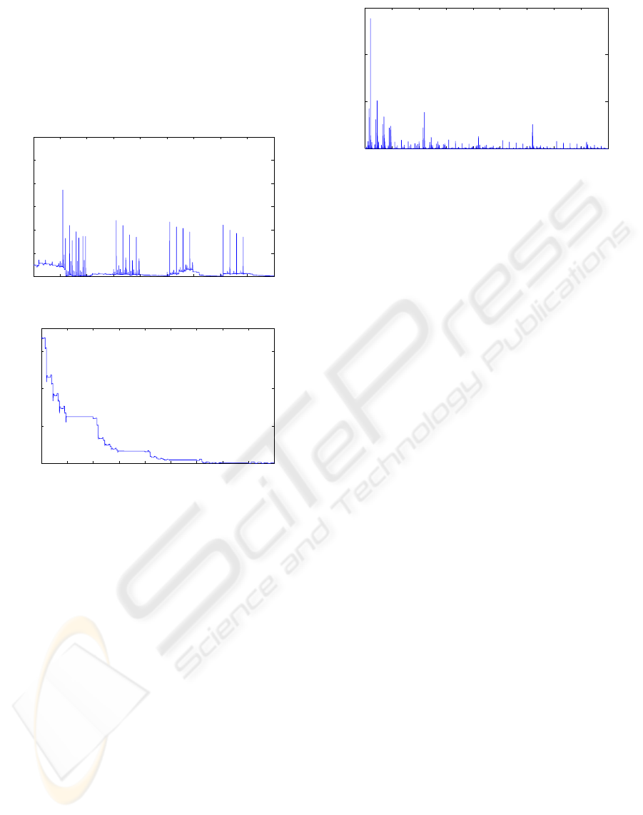
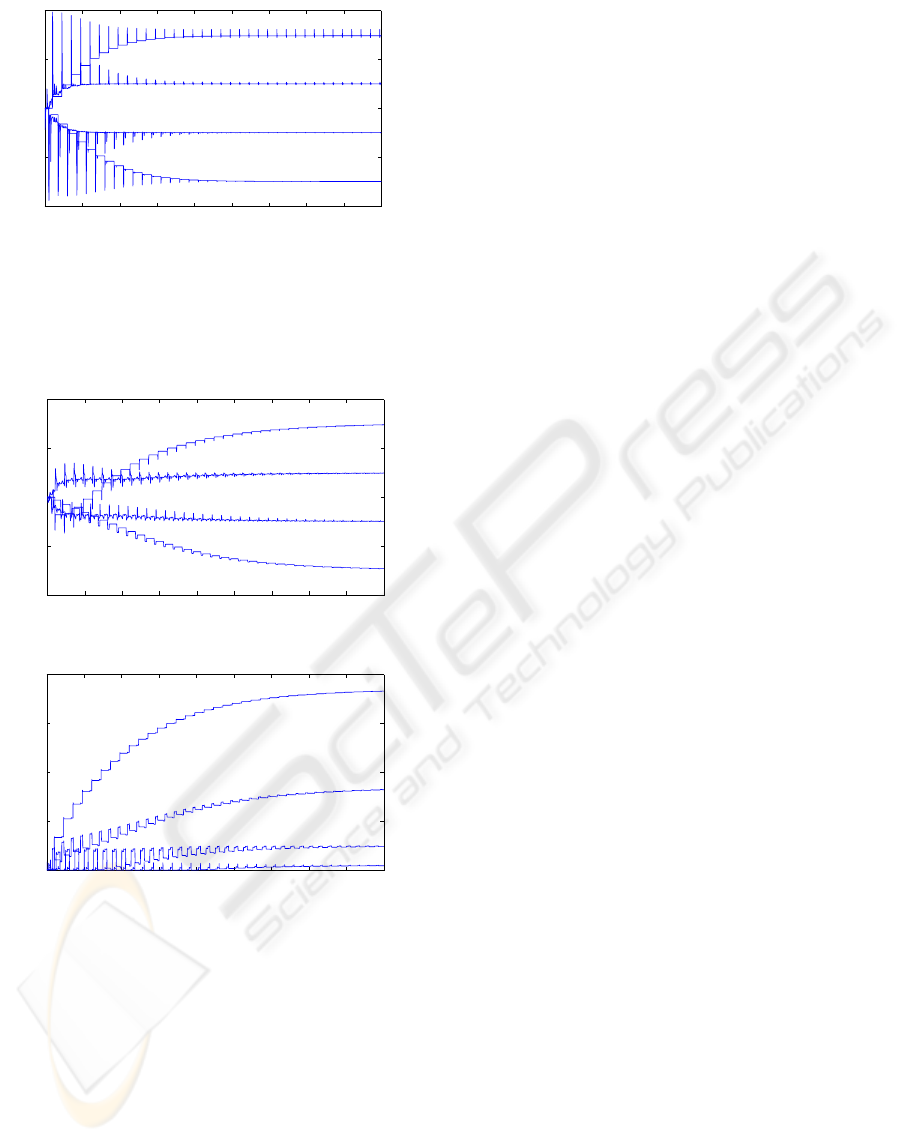
One can see in Fig. 7 that the parameter errors
quickly converge to zero. Also the tracking error con-
verges to zero as it can be seen in Fig. 8, but in the
first phase of the adaptation it is higher than in the
previous cases. We can say that the price for better
identification is a worse control performance in terms
of tracking error, at least in the initial phase.
0 200 400 600 800 1000 1200 1400 1600 180
0
0
10
20
30
40
50
60
t [s]
γ
f
Vf
(a) γ
f
Vf
0 200 400 600 800 1000 1200 1400 1600 180
0
0
500
1000
1500
t [s]
γ
g
Vg
(b) γ
g
Vg
Figure 7: Evolution over time of the γ
f
Vf and γ
g
Vgwith
scheduling of the learning rates.
6 DISCUSSION
From the mathematical analysis and from the sim-
ulations results presented, one can conclude that in
an indirect AFC scheme with adaptation laws derived
through Lyapunov synthesis, the tracking control and
the identification of the system dynamics are most of
the time conflicting goals. There are strong interac-
tions between the two fuzzy systems. As a conse-
quence, the adaptation works through successive ad-
justments: the changes in one of the fuzzy system try
to compensate the changes in the other. This interplay
can hamper the learning process, which becomes non-
monotonous. Some works related to this topic can
also be found in the standard system-identification lit-
erature.
In the context of ‘closed-loop system identifica-
tion’, and ‘identification for control’ (Landau, 1999;
0 200 400 600 800 1000 1200 1400 1600 180
0
0
0.5
1
1.5
t [s]
Ve
Figure 8: Evolution of Ve.
Hof and Schrama, 1995) it is stated that with stan-
dard identification and control design methods it is
not possible to simultaneously optimize both the sys-
tem model and the controller. Hence, in identification
for control, system identification and control design
are not simultaneous; instead they are temporally sep-
arated. System dynamics are identified in closed-loop
in the presence of a fixed controller and then, based
on the identified model, a new controller is designed.
These steps can be repeated. The analysis carried out
in this paper suggests that the separation of identifi-
cation and control may be beneficial in the context of
AFC. In (Hojati and Gazor, 2002), it is proven that
adaptive laws driven by two sources of information,
namely tracking error and prediction error (defined
with regard to a series-parallel identification model)
outperform adaptive laws based only on tracking er-
ror.
In this paper, the learning rates are abruptly
switched. With regard to stability, it may be better to
have a smooth transition of the learning rates. More-
over, if the plant parameters are unknown but fixed,
the learning rate should decrease over time (only
plants with time-varying parameters require constant
learning rates). In the literature on reinforcement
learning and neural networks, some heuristics for
the choice of learning rates are provided (Sutton and
Barto, 1998; Jacobs, 1988).
7 CONCLUSIONS
The main contribution of this paper is the analysis
of interactions between parameter updates of the two
fuzzy systems constituting an indirect adaptive fuzzy
controller based on feedback linearization. First, it
has been shown analytically what are the relation-
ships among the time-derivative of the norm of the
tracking error and of the parameter errors with re-
gard to the unknown system dynamics. The analy-
sis highlights the existence of conflicting goals: the
PARAMETER CONVERGENCE IN ADAPTIVE FUZZY CONTROL
141

identification of the unknown system dynamics and
tracking control cannot be simultaneously optimized.
Then by means of simulations with a second order
system, under different scenarios, the mathematical
developments are validated. The links with the re-
lated literature have been explored and finally some
possible improvements were suggested. In particu-
lar, we propose the scheduling of the learning rates as
possible means to overcome some parameter conver-
gence problems, simultaneously achieving the control
goal while performing a proper identification of fuzzy
models, which are fully transparent and amenable to
off-line interpretation.
REFERENCES
Chen, B. S., Lee, C. H., and Chang, Y. C. (1996). H
∞
track-
ing design of uncertain nonlinear siso systems: Adap-
tive fuzzy approach. IEEE Trans. on Fuzzy Systems,
4(1):32–43.
Fishle, K. and Schroder, D. (1999). An improved adaptive
fuzzy control method. IEEE Trans. on Fuzzy Systems,
7(1):27–40.
Han, H., Su, C. Y., and Stepanenko, Y. (2001). Adap-
tive control of a class of nonlinear systems with non-
linearly parameterized fuzzy approximators. IEEE
Trans. on Fuzzy Systems, 9(2):315–323.
Hof, P. M. J. V. D. and Schrama, R. J. P. (1995). Identi-
fication and control-closed-loop issues. Automatica,
31(12):1751–1770.
Hojati, M. and Gazor, S. (2002). Hybrid adaptive fuzzy
identification and control of nonlinear systems. IEEE
Trans. on Fuzzy Systems, 10(2):198–210.
Jacobs, R. A. (1988). Increased rates of convergence
through learning rate adaptation. Neural Networks,
1:295–307.
Landau, I. D. (1999). From robust control to adaptive con-
trol. Control Engineering Practice, (7):1113–1124.
Ordonez, R. and Passino, K. M. (1999). Stable multi-input
multi-output adaptive fuzzy/neural control. IEEE
Trans. on Fuzzy Systems, 7(3):345–353.
S. Tong, J. T. and Wang, T. (2000). Fuzzy adaptive control
of multivariable nonlinear systems. Fuzzy Sets and
Systems, (111):153–167.
Spooner, J. T. and Passino, K. M. (1996). Stable adap-
tive control using fuzzy systems and neural networks.
IEEE Trans. on Fuzzy Systems, 4(3):339–359.
Su, C. Y. and Stepanenko, Y. (1994). Adaptive control of
a class of nonlinear systems with fuzzy logic. IEEE
Trans. on Fuzzy Systems, 2(4):285–294.
Sutton, R. S. and Barto, A. G. (1998). Reinforcement Learn-
ing: an Introduction. MIT Press.
Tong, S. and Chai, T. (1999). Indirect adaptive control and
robust analysis for unknown multivariable nonlinear
systems with fuzzy logic systems. Fuzzy Sets and Sys-
tems, (106):309–319.
Tong, S., Wang, T., and Tang, J. T. (2000). Fuzzy adaptive
output tracking control of nonlinear systems. Fuzzy
Sets and Systems, (111):169–182.
Tsay, D. L., Chung, H. Y., and Lee, C. J. (1999). The adap-
tive control of nonlinear systems using the sugeno-
type of fuzzy logic. IEEE Trans. on Fuzzy Systems,
7(2):225–229.
Wang, C. H., Liu, H. L., and Lin, T. C. (2002). Direct adap-
tive fuzzy-neural control with state observer and su-
pervisory controller for unkown nonlinear dynamical
systems. IEEE Trans. on Fuzzy Systems, 10(1):39–49.
Wang, L. X. (1993). Stable adaptive fuzzy control of nonlin-
ear systems. IEEE Trans. on Fuzzy Systems, 1(2):146–
154.
Wang, L. X. (1994). Adaptive Fuzzy Systems and Control:
Design and Stability Analysis. Prentice-Hall.
Wang, L. X. (1996). Stable adaptive fuzzy controllers
with application to inverted pendulum tracking. IEEE
Trans. on Systems, Man, and Cybernetics, 26(5):677–
691.
ICINCO 2004 - INTELLIGENT CONTROL SYSTEMS AND OPTIMIZATION
142
