
DYNAMIC STRUCTURE CELLULAR AUTOMATA
IN A FIRE SPREADING APPLICATION
Alexandre Muzy, Eric Innocenti, Antoine Aïello, Jean-François Santucci, Paul-Antoine Santoni
University of Corsica
SPE – UMR CNRS 6134
B.P. 52, Campus Grossetti, 20250 Corti. FRANCE.
David R.C. Hill
ISIMA/LIMOS UMR CNRS 6158
Blaise Pascal University
Campus des Cézeaux BP 10125, 63177 Aubière Cedex. FRANCE.
Keywords: Systems modeling, Discrete event systems, Multi-formalism, Fire spread, cellular automata.
Abstract: Studying complex propagation phenomena is usually
performed through cellular simulation models.
Usually cellular models are specific cellular automata developed by non-computer specialists. We attempt
to present here a mathematical specification of a new kind of CA. The latter allows to soundly specify
cellular models using a discrete time base, avoiding basic CA limitations (infinite lattice, neighborhood and
rules uniformity of the cells, closure of the system to external events, static structure, etc.). Object-oriented
techniques and discrete event simulation are used to achieve this goal. The approach is validated through a
fire spreading application.
1 INTRODUCTION
When modeling real systems, scientists cut off
pieces of a biggest system: the world surrounding us.
Global understanding of that world necessitates
connecting all these pieces (or subsystems),
referencing some of them in space. When the whole
system is complex, the only way to study its
dynamics is simulation.
Propagation phenomena as fire, swelling, gas
propagation,
(…) are complex systems. Studying
these phenomena generally leads to divide the
propagation space in cells, thus defining a cellular
system.
Developed from the General Systems Theory
(M
esarovic and Takahara, 1975), the Discrete Event
Structure Specification (DEVS) formalism (Zeigler
et al., 2000) offers a theoretical framework to map
systems specifications into most classes of
simulation models (differential equations,
asynchronous cellular automata, etc.). For each
model class, one DEVS sub-formalism will allow to
faithfully specify one simulation model. As
specification of complex systems often needs to
grasp different kinds of simulation models,
connections between the models can be performed
using DEVS multi-formalism concepts.
Another DEVS advantage relates to its ability in
pr
oviding discrete event simulation techniques, thus
enabling to concentrate the simulation on active
components and resulting in performance
improvements.
Precise and sound definition of propagation
need
s to use models from physics as Partial
Differential Equations (PDEs). These equations are
then discretized leading to discrete time simulation
models. These models are generally simulated from
scientists by using specific Cellular Automata (CA).
As defined in (Wolfram, 1994), standard CA consist
of an infinite lattice of discrete identical sites, each
site taking on a finite site of, for instance, integer
values. The values of the sites evolve in discrete
143
Muzy A., Innocenti E., Aïello A., Santucci J., Santoni P. and C. Hill D. (2004).
DYNAMIC STRUCTURE CELLULAR AUTOMATA IN A FIRE SPREADING APPLICATION.
In Proceedings of the First International Conference on Informatics in Control, Automation and Robotics, pages 143-151
DOI: 10.5220/0001129801430151
Copyright
c
SciTePress
time steps according to deterministic rules that
specify the value of each site in terms of the values
of neighboring sites. CA may thus be considered as
discrete idealizations of PDEs. CA are models where
space, time and states are discrete (Jen, 1990).
However, definition of basic CA is too limited to
specify complicated simulations (infinite lattice,
neighborhood and rules uniformity of the cells,
closure of the system to external events, discrete
state of the cells, etc.). Scientists often need to
modify CA’s structure for simulation purposes
(Worsch, 1999).
We extend here basic CA capabilities by using
object-oriented techniques and discrete event
simulation (Hill, 1996). A mathematical
specification of the approach is defined using the
Dynamic Structure Discrete Time System
Specification (DSDTSS) formalism (Barros, 1997).
This formalism allows dynamically changing the
structure of discrete time systems during the
simulation. These new CA are called the Dynamic
Structure Cellular Automata (DSCA).
DSCA have been introduced in (Barros and
Mendes, 1997) as a formal approach allowing to
dynamically change network structures of
asynchronous CA. Using an asynchronous time
base, cells were dynamically instantiated or
destroyed during a fire spread simulation.
The scope here is to extend basic CA capabilities
using a discrete time base. If previous DSCA were
dedicated to discrete event cellular system
specification, we extend here the DSCA definition to
discrete time cellular system specification.
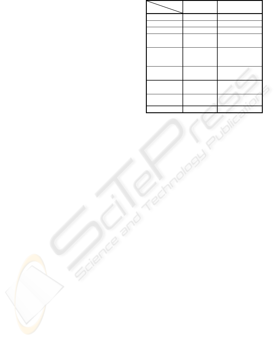
Table 1 sums up the advantages of the DSCA in
relation to basic CA. In DSCA, each cell can contain
different behaviors, neighborhoods and state
variables. Rules and neighborhoods of the cells can
dynamically change during the simulation. Each cell
can receive external events. During the simulation,
the computing of state changes is limited to active.
Finally, a global transition function allows the
specification of the DSCA global behaviors.
Table 1: DSCA extensions
Basic CA DSCA
Time discrete Discrete
Space discrete Discrete
State discrete Continuous
Closure to
external events
- +
Different
variables per
cell
- +
Rules
uniformity*
- +
Neighborhood
uniformity*
- +
Activity
tracking*
-
+
Global function - +
*at simulation time
The DSCA definition is validated against a fire
spreading application. Recent forest fires in Europe
(Portugal, France and Corsica) and in the United
States (California) unfortunately pinpoint the
necessity of increasing research efforts in this
domain. Fires are economical, ecological and human
catastrophes. Especially as we know that present
rising of wild land surfaces and climate warming
will increase forest fires.
Modeling such a huge and complex phenomenon
obviously leads to simulation performance
overloadings and design problems.
Simulation model reusability has to face to the
complicated aspects of both model implementations
and model modifications. Despite a large number of
cells, simulation has to respect real time deadlines to
predict actual fire propagations. Hence, this kind of
simulation application provides a powerful
validation to our work.
This study is organized as follows. First some
formalisms background is provided. Then two
sections present the DSCA modeling and simulation
principles. After, simulation results of a fire
spreading application are provided. Finally, we
conclude and make some prospects.
2 BACKGROUND
A formalism is a mathematical description of a
system allowing to guide a modeler in the
specification task. The more a formalism fits to a
system class, the more simple and accurate it will be.
Efficiently modeling complex systems often
implies the need to define subsystems using different
ICINCO 2004 - SIGNAL PROCESSING, SYSTEMS MODELING AND CONTROL
144

formalisms. Connections between the different
formalisms can then be achieved through a multi-
formalism to perform the whole system
specification.
In this study, subsystems are specified using
DEVS, DTSS (Discrete Time System Specification)
and DSDTSS formalisms. Connections between the
different models are achieved using a Multi-
formalism Network (MFN). A structure description
of each model is provided hereafter.
A DEVS atomic model is a structure:
DEVS = (X, Y, Q, q
0
, δ
int
, δ
ext
, λ, t
a
)
where X is the input events set, Q is the set of state,
q
0
is the initial state, Y is the output events set, δ
int
:
Q
Æ
Q is the internal transition function, δ
ext
: Q×X
Æ
Q is the external transition function,
λ
: Q
Æ
Y
the output function, t
a
is the time advance function.
DSDTSS basic models are DTSS atomic model:
DTSS = (X, Y, Q, q
0
,
δ
,
λ
, h)
where X, Y are the input and output sets, Q is the
set of state, q
0
is the initial state,
δ
: Q×X
Æ
Q is
the state transition function,
λ
: Q
Æ
Y is the
output function (considering a Moore machine) and
h is a constant time advance.
At a periodic rate, this model checks its inputs
and, based on its state information, produces an
output and changes its internal state.
The network of simple DTSS models is referred
to as a Dynamic Structure Discrete Time Network
(DSDTN) (Barros, 1997). We introduce here input
and output sets to allow connections with the
network. Formally, a DSDTN is a 4-tuple:
DSDTN = (X
DSDTN
,Y
DSDTN
,
χ
, M
χ
)
where X
DSDTN
is the network input values set, Y
DSDTN
is the network input values set,
χ
is the name of the
DSDTN executive, M
χ
is the model of the executive
χ
.
The model of the executive is a modified DTSS
defined by the 8-tuple:
M
χ
= (X
χ
,Q
χ
, q
0,
χ
, Y
χ
,
γ
,
Σ
*
,
δ
χ
,
λ
χ
)
where
γ
: Q
χ
Æ
Σ
*
is the structure function, and
Σ
*
is
the set of network structures. The transition function
δ
χ
computes the executive state q
χ
. The network
executive structure
Σ
, at the state q
χ
∈
Q
χ
is given by
Σ
=
γ
(q
χ
) = (D, {M
i
}, {I
i
}, {Z
i,j
}), for all i
∈
D, M
i
=
(X
i
, Q
i
, q
0,i
, Y
i
,
δ
i
,
λ
i
), where D is the set of model
references, I
i
is the set of influencers of model i, and
Z
i,j
is the i to j translation function.
Because the network coupling information is
located in the state of the executive, transition
functions can change this state and, in consequence,
change the structure of the network. Changes in
structure include changes in model interconnections,
changes in system definition, and the addition or
deletion of system models.
Formally, a multiformalism network (Zeigler et
al., 2000) is defined by the 7-tuple:
MFN = (X
MFN
,Y
MFN
, D, {M
i
}, {I
i
}, {Z
i,j
},select)
where X
MFN
=X
discr
×X
cont
is the network input values
set, X
discr
and X
cont
are discrete and continuous input
sets, Y
MFN
=Y
discr
×Y
cont
is the network input values
set, Y
discr
and Y
cont
are discrete and continuous output
sets, D is the set of model references,
For each i
∈
D,
M
i
is are DEVS, DEVN, DTSN, DTSS,
DESS, DEV&DESS or other MFN models.
As DSDTSS proved to be closed under
coupling, M
i
can also be dynamic structure
models or networks,
I
i
is the set of influencers of model i,
Z
i,j
is the i to j translation function,
select is the tie-breaking function.
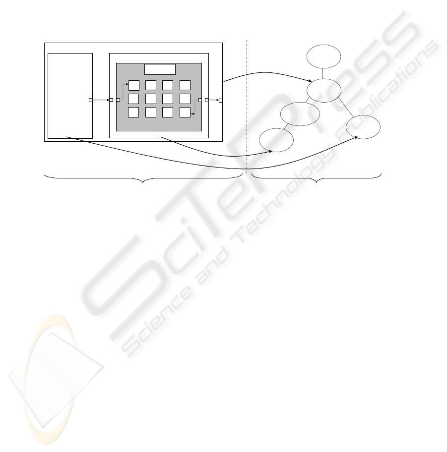
3 DSCA MODELLING
Models composing a DSCA are specified here using
the previous model definitions. As described in the
modeling part of Figure 1, external events are
simulated using a DEVS atomic model: the
Generator. The latter can asynchronously generate
data information to the DSCA during the simulation.
The cell space is embedded in a DSDTN. Each cell
is defined as a DTSS model. Using its transition
function, the DSCA executive model (containing
every cells) achieves changes in structure directly
accessing to the attributes of cells. A mathematical
description of each model is provided here after.
We define the MFN by the structure:
MFN = (X
MFN
,Y
MFN
, D, {M
i
}, {I
i
}, {Z
i,j
}, select)
where D={G,DSDTN}, M
G
= (X
G
, Q
G
, q
0,G
, Y
G
,
δ
G
,
λ
G,
τ
G
), M
DSDTN
=DSDTN, I
G
={}, I
DSDTN
={G}, and
Z
DSDTN,MFN
: Y
DSDTN
Æ
Y
MFN
, Z
G,DSDTN
: Y
G
Æ
X
DSDTN
.
DYNAMIC STRUCTURE CELLULAR AUTOMATA IN A FIRE SPREADING APPLICATION
145

We define the DSDTN by the structure:
DSDTN = (X
DSDTN
, Y
DSDTN
, DSCA, M
DSCA
)
where
Σ
=
γ
(q
0
,
χ
) = (D, {M
i
}, {I
i
}, {Z
i,j
}), where
D={(i,j) / (i,j)
∈
}, M
2
ℑ
DSCA
= (X
DSCA
, Q
DSCA
,
q
0,DSCA
, Y
DSCA
,
δ
DSCA
,
λ
DSCA
), I
DSCA
={DSDTN},
I
cell
={cell
n
,DSDTN}. Where I
cell
= {I
kl
/ k
∈
[0,m], l
∈
[0,n]} is the neighbourhood set (or the set of
influencers) of the cell as defined in (Wainer and
Giambiasi, 2001). It is a list of pairs defining the
relative position between the neighbours and the
origin cell. I
kl
= {(i
p
,j
p
) /
∀
p
∈
I
cell
, p
∈
[1,η
kl
], i
p
,j
p
∈
Z ; |k- i
p
| ≥ 0 |l- j∧
p
| ≥ 0 ∧ η
kl
∈
I
cell
}, and η
∈
I
cell
is the neighborhood size.
Z
cell,DSCA
: Y
cell
ÆY
DSCA
, Z
DSCA,DSDTN
:
Y
DSCA
ÆY
DSDTN
, Z
DSDTN,DSCA
: X
DSDTN
ÆX
DSCA
,
Z
DSCA,cell
: X
DSCA
Æ
X
cell
.
For the implementation, ports are defined:
Py
G
=Px
DSDTN
=Px
DSCA
={data}
Py
DSCA
=Py
DSDTN
=Py
MFN
={state}
Px
cell
=Py
cell
={(i,j)}
We specify each cell as a special case of DTSS
model:
cell=(X
cell
, Q
cell
, q
0
,
cell
, Y
cell
,
δ
cell
,
λ
cell
)
where X
cell
is an arbitrary set of input values, Y
cell
is
an arbitrary set of output values, q
0,cell
is the initial
state of the cell and
q
∈
Q
cell
is given by:
q=((i,j), state, N, phase),
(i,j)
∈
, is the position of the cell,
2
ℑ
state is the state of the cell,
N
= {N
kl
/ k
∈
[0,m], l
∈
[0,n]}. N is a list of
states N
kl
of the neighboring cells of coordinates
(k,l),
phase = {passive, active} corresponds to the
name of the corresponding dynamic behavior.
For numerous adjacent active cells, the active
phase can be decomposed in ‘testing’ and
‘nonTesting’ phases. The use of these phase is
detailed in section 5.
δ
cell
: Q
cell
×X
cell
Æ
Q
cell
λ
cell
: Q
cell
Æ
Y
cell
4 DSCA SIMULATION
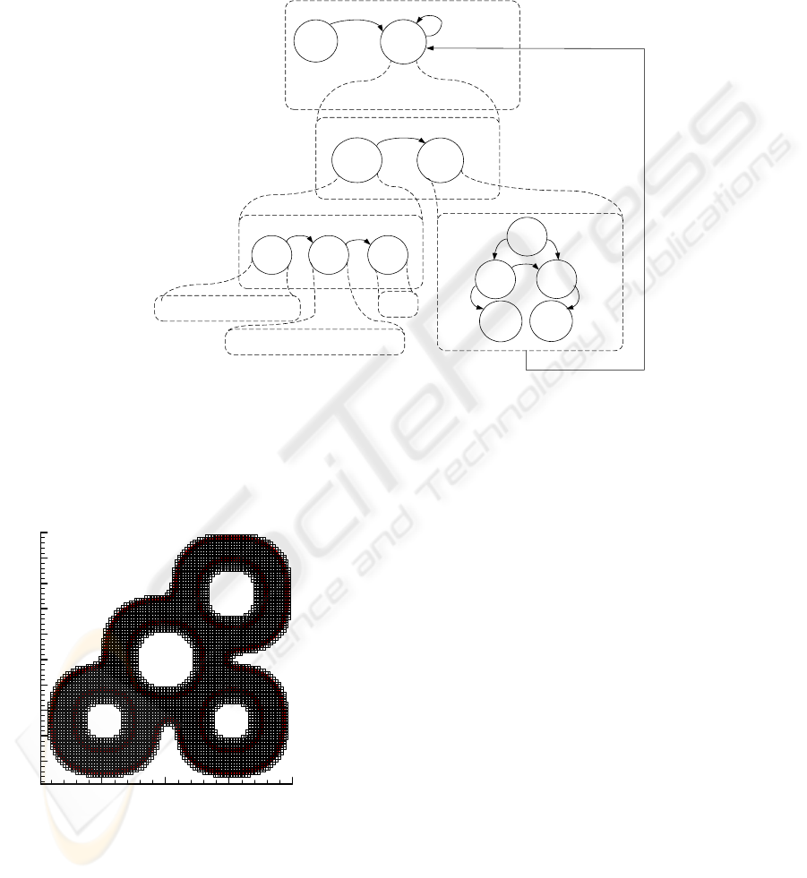
As depicted in Figure 2, implementation of discrete
event models consists in dividing a transition
function
δ
d
of a model according to event types ev
n
issued from a set of possible event types S
d
. The
transition function then depends on the event types
the model receives.
Model d
S
d
= {ev
1
, ev
2
, … , ev
n
}
δ
d
(S
d
)
case S
d
ev
1
: call event-routine
1
ev
2
: call event-routine
2
…
ev
n
: call event-routine
n
Figure 2: Discrete event model implementation
(Zeigler et al., 2000)
The DSCA receives data from the Generator.
These data represent external influences of the
DSCA. During the simulation, information is
embedded in messages and transits through the data
and state ports. Messages have fields [Message type,
Time, Source processor, Destination port, Content],
where Content is a vector of triplets [Event type,
Value, Coordinate port]. When a DSCA receives a
message on its data port, the corresponding
Aggregated Network Simulator (AN Simulator)
scans the Content vector and according to the
Coordinate port, sends the [Event type, Value] pairs
to the concerned cells. A vector of pairs [Event type,
Value] can be sent to a cell port. Then, according to
the Event type a cell receives, it will update the
concerned attributes, executing the concerned
transition function.
The simulation tree hierarchy is described in the
simulation part on the right side of Figure 1. Except
for the Root and DTSS interface, all nodes of the tree
are processors attached to models. The processors
manage with message exchanges and execution of
model functions. Each processor is automatically
generated when the simulation starts.
The Coordinator pilots the MFN model, the
simulator SimG pilots the Generator, the DSDTN
model and the DSDTN models are piloted by the
Aggregated Network Simulator (AN Simulator).
Algorithms of the DSCA simulators can be found in
(Muzy et al., 2003). Algorithms of basic DEVS
simulators and DTSS interfaces can be found in
(Zeigler et al., 2000).
The Root processor supervises the whole
simulation loop. It updates the simulation time and
activates messages at each time step. For the
Coordinator, the DTSS interface makes the
Aggregated Network simulator seen as a DEVS
atomic simulator. This is done by storing all
messages arriving at the same time step and then by
calculating the new state and output of the DSCA
ICINCO 2004 - SIGNAL PROCESSING, SYSTEMS MODELING AND CONTROL
146
when receiving an internal transition message. The
simulation tree thus respects the DEVS bus
principle. That means that whatever DEVS model
can be appended to the simulation tree.
5 ACTIVITY TRACKING
Using discrete event cellular models, activity
tracking can be easily achieved (Nutaro et al., 2003).
Active cells send significant events to be reactivated
or to activate neighbors at next time step. However,
pure discrete event models proved to be inefficient
for discrete time system simulation (Muzy et al.,
2002). Interface configurations and message
management produce simulation overheads,
especially for numerous active components.
For discrete time systems, we know that each
component will be activated at each time step.
Moreover, in CA, states of cells directly depend on
the states of their neighbors. To optimize the
simulation, messages between the cells have to be
canceled and simulation time advance has to be
discrete. However, a new algorithm has to be
defined to track active c
ells.
Coordinator
SimG
DTSS-interface
Root
AN Simulator
DSDTN
MFN
Generator
data data
state
s
DSCA
Cell
…
states
(0,0)
(m,n)
modelling simulation
Figure 1: DSCA modeling and simulation
To focus the simulation on active cells, we use
the basic principles exposed in (Zeigler et al.,
2000) to predict whether a cell will possibly
change state or will definitely be left unchanged in
a next global state transition: “a cell will not
change state if none of its neighboring cells
changed state at the current state transition time”.
Nevertheless, to obtain optimum performance
the entire set of cells cannot be tested. Thereby, an
algorithm, which consists in testing only the
neighborhood of the active bordering cells of a
propagation domain, has been defined for this type
of phenomena.
To be well designed, a simulation model should
be structured so that all information relevant to a
particular design can be found in the same place.
This principle enhances models modularity and
reusability making easier further modifications.
Pure discrete event cells are all containing a
micro algorithm, which allows to focus the whole
simulation loop on active cells. We pinpointed
above the inefficiency of such an implementation
for discrete time simulation. An intuitive and
efficient way to achieve activity tracking in
discrete time simulation is to specify this particular
design at one place. As depicted in Figure 3, the
activity tracking algorithm is located in the global
transition function of the DSCA, in charge of the
structure evolution of the cell space.
Cells are in ‘testing’ phases when located at the
edge of the propagation domain, ‘nonTesting’
when not tested at each state transition and
‘quiescent’ when inactive.
A propagation example is sketched in Figure 4
for cardinal and adjacent neighborhoods. In our
algorithm, only the bordering cells test their
neighborhood, this allows to reduce the number of
testing cells.
The result of the spreadTest(i,j,nextState)
function of Figure 3, depends on the state of the
tested cells. If this state fulfils a certain condition
defined by the user, the cell becomes ‘nonTesting’
and new tested neighboring are added to the set of
active cells. The transition function receives x
χ
messages from the Generator corresponding to
external events. The x
χ
messages contain the
coordinates of the cells influenced by the external
event. If the coordinates are located in the domain
DYNAMIC STRUCTURE CELLULAR AUTOMATA IN A FIRE SPREADING APPLICATION
147
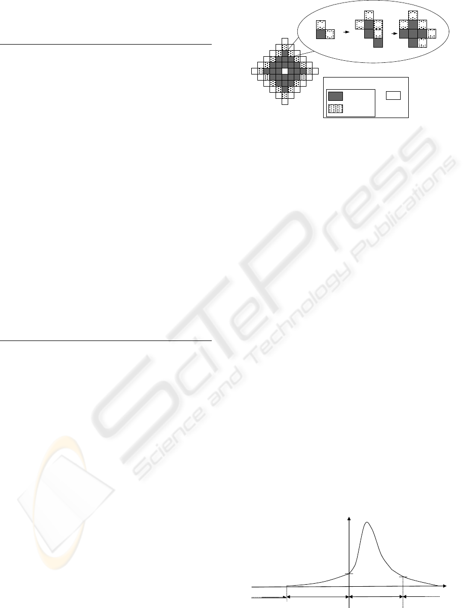
calculation, the state of the cell is changed by
activating its transition function with the new
value. Otherwise, new cells are added to the
propagation domain.
t
t+h
t+2h
?
?
?
?
??
??
?
?
?
quiescent
non testing
testing
active
//’Q’ is for the quiescent phase,
//’T’ for the testing one and ‘N’ for
//the nonTesting one
Transition Function(x
χ
)
For each cell(i,j) Do
If(cellPhase(i,j)==’Q’) Then
removeCell(i,j)
Endif
If(cellPhase(i,j)==’T’) Then
If (cellNearToBorder(i,j)) Then
setSpreadStateCell(i,j,’N’)
Else
If(spreadTest(i,j,nextState))Then
setCellPhase(i,j,‘N’)
addQuiescentNeighboringCells(i,j)
EndIf
EndIf
EndIf
EndFor
If(x
χ
message is not empty)
If(cells in the propagation domain) Then
cell(i,j).transitionF(newState)
change the cell states //
Else
addNewCells()
EndIf
EndIf
EndTransitionFunction()
Figure 3: Transition function of the DSCA
For efficiency reasons, the simulation engine
we developed has been implemented in C++ and
dynamic allocation has been suppressed for some
classes. Indeed, for significant numbers of object
instantiation/deletion dynamic allocation is
inefficient and we have designed a specialized
static allocation (Stroustrup, 2000). A pre-
dimensioning via large static arrays can be easily
achieved thanks to current modern computer
memory capabilities.
The state of the executive model is a matrix of
cellular objects. References on active cells are
stored in a vector container. A start-pointer and an
end-pointer are delimiting the current calculation
domain on the vector. Thus initial active cells that
are completely burned during a simulation run can
be dynamically ignored in the main loop. At each
time step, by modifying the position of pointers,
new tested cells can be added to the calculation
domain and cells that return in a quiescent state are
removed from the former.
Figure 4: Calculation domain evolution
6 FIRE SPREADING
APPLICATION
The simulation engine we use has been proved to
achieve real-time simulation (Muzy et al., 2003).
Moreover, we use a mathematical fire spread
model already validated and presented in (Balbi et
al., 1998). In this model, a Partial Differential
Equation (PDE) represents the temperature of each
cell. A CA is obtained after discretizing the PDE.
Using the finite difference method leads to the
following algebraic equation:
(1)
k
ji
tt
v
k
ji
k
ji
k
ji
k
ji
k
ji
dTeTTbTTaT
ig
,
)(
0,1,1,,1,1
1
,
)()( +++++=
−−
+−+−
+
α
σ
where T
ij
is the grid node temperature. The
coefficients a, b, c and d depend on the time step
and mesh size considered, t is the real time, t
ig
the
real ignition time (the time the cell is ignited) and
σ
ν
,0
is the initial combustible mass.
Figure 5 depicts a simplified temperature curve
of a cell in the domain. We consider that above a
threshold temperature T
ig
, the combustion occurs
and below a temperature T
f
, the combustion is
finished.
The end of the real curve is purposely neglected
to save simulation time. Four states corresponding
to the behavior of each cell behavior are defined
from these assumptions. The four states are:
‘unburned’, ‘heating’, ‘onFire’ and ‘burned’.
t
(Ta, tig)
Tf = 333 K
Tig = 573 K
T (Kelvin)
heating
burned
onFire
unburned
Figure 5: Simplified temperature curve of a cell behavior
ICINCO 2004 - SIGNAL PROCESSING, SYSTEMS MODELING AND CONTROL
148
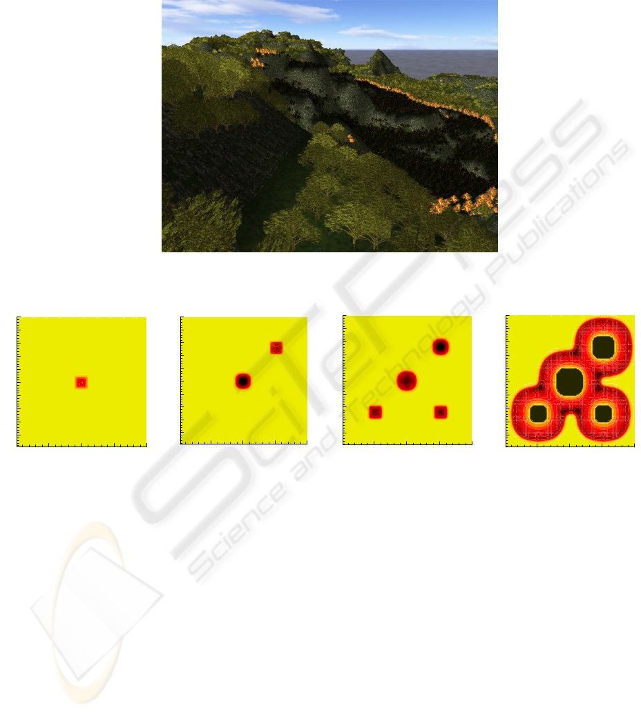
Figure 6 depicts a fire spreading in a Corsican
valley, generated using the OpenGL graphics
library. By looking at this picture we easily
understand that simulation has to focus only on a
small part of the whole land. Actually, areas of
activity just correspond to the fire front, and to the
cells in front of the latter (corresponding to cells in
one of the following states: ‘heating’ or ‘onFire’ ).
Figure 6:
3D Visualization of fire spreading
X(cells)
Y(cells)
25 50 75 10
0
10
20
30
40
50
60
70
80
90
100
X
(
c
e
l
l
s
)
Y(cells)
25 50 75 100
10
20
30
40
50
60
70
80
90
100
X(cells)
Y(cells)
25 50 75 100
10
20
30
40
50
60
70
80
90
100
X(cells)
Y(cells)
25 50 75 10
0
10
20
30
40
50
60
70
80
90
100
Figure 7: Fire ignitions and propagation
During a fire spreading, flying brands ignite
new part of lands away from the fire. This is an
important cause of fire spreading. However,
tracking activity of flying brands is difficult.
Firstly, because flying brands occur whenever
during the simulation time. Secondly, because they
occur far away from the calculation domain, thus
new calculation allocations need to be created
dynamically.
Figure 7 represents a case of multi-ignitions
during the simulation. Simulation starts with one
ignition on the center of the propagation domain.
Then, at time t=7s, a second ignition occurs on the
top right corner of the propagation domain.
Finally, at t=12s, two new ignitions occur on the
right and left bottom of the propagation domain.
The last picture shows the multiple fire fronts
positions at t=70s.
Figure 8 describes the DSCA state transitions in
a fire spread simulation. First the simulation starts
with the first ignition, which is simulated by an
output external event of the Generator of Figure 1.
Then the main simulation loop calculating the fire
front position is activated. The latter consists in
calculating the temperature of cells. After,
according to the calculated temperatures, the
calculation domain is updated. For each cell of the
calculation domain, the temperature is calculated
using equation (1), according to the state of the
cells. The calculation domain is updated using the
algorithm described in Figures 3 and 4. Phase
transitions depend on the temperature of cells.
At the initialization, only one calculation
domain corresponding to the one described in
Figure 4 is generated. Bordering cells of the
calculation domain are in a ‘testing’ phase and
DYNAMIC STRUCTURE CELLULAR AUTOMATA IN A FIRE SPREADING APPLICATION
149
non-bordering cells in a ‘nonTesting’ one.
Remaining cells are ‘quiescent’. If the temperature
of a ‘testing’ cell fulfills a certain threshold
temperature T
t
, the testing cell will pass in the
‘nonTesting’ phase and neighboring ‘testing’ cells
will be added to the calculation domain. In the fire
spread case, this threshold can be fixed slightly
over the ambient temperature.
During the simulation, the Generator simulates
the flying brands by sending external events. When
the DSCA receives the events and updates the
calculation domain.
ignition
!endSimulationTime
or
!inactivity
igniting
activity
tracking
new cells'
temperature
inactive
testing
non
testing
remove
cell
add
neighbors
unburned
burning
burned
bordering cell non bordering cell
T <= TfT >= Tt
T >= Tig
T <= Tf
T >= Tt
k
ji
k
ji
k
ji
k
ji
k
ji
k
ji
dTTTbTTaT
,1,1,,1,1
1
,
)()( ++++=
+−+−
+
)(
0,1,1,,1,1
1
,
.)()(
tigtk
ji
k
ji
k
ji
k
ji
k
ji
k
ji
edTTTbTTaT
−−
+−+−
+
+++++=
α
υ
σ
aji
TT =
,
calculating
cells'
temperature
Calculating
flame front
position
Internal input
ttt
∆
+
=
Figure 8: Transition state diagram
The resulting activity tracking is showed in
Figure 9. We can notice that active cells
correspond to the fire front lines, not to the burned
and non-heated areas.
Figure 9: Activity tracking
7 CONCLUSION
Considering the previous discrete event DSCA
(Barros and Mendes, 1997), new well-designed
and complementary discrete time DSCA have been
defined here. These two methodologies allow to
faithfully guide modelers for modeling and
simulating discrete event and discrete time cellular
simulation models.
X(cells)
Y(cells)
25 50 75 100
10
20
30
40
50
60
70
80
90
100
DSCA allow to simulate a large range of
complicated cellular models. Complex phenomena
can be simulated thanks to basic CA simplicity.
We hope that even more complex phenomena will
be able to be simulated thanks to DSCA. To be
well understood and widely applied, DSCA
definition has to be as clear and simple as possible.
Clearness and simplification of DSCA
specification will remain our objective.
Another objective will be to improve DSCA
specification using new experiments. To achieve
this goal, complexity of fire spread remains an
infinite challenge for DSCA simulation. We plan
now to extend the DSCA specification to the
simulation of implicit-time models.
Another important validation of our approach
concerns network structure changes. Here again, a
fire spread model taking into account wind effects
(Simeoni et al., 2003) will allow us to validate
DSCA network structure changes. This model
actually needs to dynamically change the
ICINCO 2004 - SIGNAL PROCESSING, SYSTEMS MODELING AND CONTROL
150

neighborhood of burning cells according to the fire
front shape.
ACKNOWLEDGMENTS
We would like to thank our research assistant
Mathieu Joubert, for his technical support and for
his C++ implementation of the 3D visualization
tool using OpenGL.
REFERENCES
Balbi, J. H., P. A. Santoni, and J. L. Dupuy, 1998.
Dynamic modelling of fire spread across a fuel bed.
Int. J. Wildland Fire, p. 275-284.
Barros, F. J., 1997. Modelling Formalisms for Dynamic
Structure Systems. ACM Transactions on Modelling
and Computer Simulation, v. 7, p. 501-515.
Barros, F. J., and M. T. Mendes, 1997. Forest fire
modelling and simulation in the DELTA
environment. Simulation Practice and Theory, v. 5,
p. 185-197.
Hill, D. R. C., 1996. Object-oriented analysis and
simulation, Addison-Wisley Longman, UK, 291 p.
Jen, E., 1990. A periodicity in one-dimensional cellular
automata. Physica, v. 45, p. 3-18.
Mesarovic, M. D., and Y. Takahara, 1975. General
Systems Theory: A mathematical foundation,
Academic Press. New York.
Muzy, A., E. Innocenti, F. Barros, A. Aïello, and J. F.
Santucci, 2003. Efficient simulation of large-scale
dynamic structure cell spaces. Summer Computer
Simulation Conference, p. 378-383.
Muzy, A., G. Wainer, E. Innocenti, A. Aiello, and J. F.
Santucci, 2002. Comparing simulation methods for
fire spreading across a fuel bed. AIS 2002 -
Simulation and planning in high autonomy systems
conference, p. 219-224.
Nutaro, J., B. P. Zeigler, R. Jammalamadaka, and S.
Akrekar, 2003. Discrete event solution of gaz
dynamics winthin the DEVS framework: exploiting
spatiotemporal heterogeneity. Intrnational
conference for computational science.
Simeoni, A., P. A. Santoni, M. Larini, and J. H. Balbi,
2003. Reduction of a multiphase formulation to
include a simplified flow
in a semi-physical model of fire spread across a fuel bed.
International Journal of Thermal Sciences, v. 42, p.
95–105.
Stroustrup, B., 2000. The C++ Programming Language,
1029 p.
Wainer, G., and N. Giambiasi, 2001. Application of the
Cell-DEVS paradigm for cell spaces modeling and
simulation. Simulation, v. 76, p. 22-39.
Wolfram, S., 1994. Cellular automata and complexity:
Collected papers, Addison-Wesly.
Worsch, T., 1999. Simulation of cellular automata.
Future Generation Computer Systems, v. 16, p. 157-
170.
Zeigler, B. P., H. Praehofer, and T. G. Kim, 2000.
Theory of modelling and simulation, Academic
Press.
DYNAMIC STRUCTURE CELLULAR AUTOMATA IN A FIRE SPREADING APPLICATION
151
