
ON MODELING AND CONTROL OF DISCRETE TIMED EVENT
GRAPHS WITH MULTIPLIERS USING (MIN, +) ALGEBRA
Samir Hamaci
Jean-Louis Boimond
S
´
ebastien Lahaye
LISA
62 avenue Notre Dame du Lac - Angers, France
Keywords:
Discrete timed event graphs with multipliers, timed weighted marked graphs, dioid, (min, +) algebra, Resid-
uation, just-in-time control.
Abstract:
Timed event graphs with multipliers, also called timed weighted marked graphs, constitute a subclass of Petri
nets well adapted to model discrete event systems involving synchronization and saturation phenomena. Their
dynamic behaviors can be modeled by using a particular algebra of operators. A just in time control method
of these graphs based on Residuation theory is proposed.
1 INTRODUCTION
Petri nets are widely used to model and analyze
discrete-event systems. We consider in this paper
timed event graphs
1
with multipliers (TEGM’s). Such
graphs are well adapted for modeling synchronization
and saturation phenomena. The use of multipliers as-
sociated with arcs is natural to model a large num-
ber of systems, for example when the achievement
of a specific task requires several units of a same re-
source, or when an assembly operation requires sev-
eral units of a same part. Note that TEGM’s can
not be easily transformed into (ordinary) TEG’s. It
turns out that the proposed transformation methods
suppose that graphs are strongly connected under par-
ticular server semantics hypothesis (single server in
(Munier, 1993), or infinite server in (Nakamura and
Silva, 1999)) and lead to a duplication of transitions
and places.
This paper deals with just in time control, i.e., fire
input transitions at the latest so that the firings of out-
put transitions occur at the latest before the desired
ones. In a production context, such a control input
minimizes the work in process while satisfying the
customer demand. To our knowledge, works on this
tracking problem only concern timed event graphs
without multipliers (Baccelli et al., 1992, §5.6), (Co-
hen et al., 1989), (Cottenceau et al., 2001).
1
Petri nets for which each place has exactly one up-
stream and one downstream transition.
TEGM’s can be handled in a particular algebraic
structure, called dioid, in order to do analogies with
conventional system theory. More precisely, we use
an algebra of operators mainly inspired by (Cohen
et al., 1998a), (Cohen et al., 1998b), and defined
on a set of operators endowed with pointwise min-
imum operation as addition and composition opera-
tion as multiplication. The presence of multipliers
in the graphs implies the presence of inferior integer
parts in order to preserve integrity of discrete vari-
ables used in the models. Moreover, the resulting
models are non linear which prevents from using a
classical transfer approach to obtain the just in time
control law of TEGM’s. As alternative, we propose a
control method based on ”backward” equations.
The paper is organized as follows. A description of
TEGM’s by using recurrent equations is proposed in
Section 2. An algebra of operators, inspired by (Co-
hen et al., 1998a), (Cohen et al., 1998b), is introduced
in Section 3 to model these graphs by using a state
representation. In addition to operators γ, δ usually
used to model discrete timed event graphs (without
multipliers), we add the operator µ to allow multi-
pliers on arcs. The just in time control method of
TEGM’s is proposed in Section 4 and is mainly based
on Residuation theory (Blyth and Janowitz, 1972).
After recalling basic elements of this theory, we recall
the residuals of operators γ, δ, and give the residual of
operator µ which involves using the superior integer
part. The just in time control is expressed as the great-
32
Hamaci S., Boimond J. and Lahaye S. (2004).
ON MODELING AND CONTROL OF DISCRETE TIMED EVENT GRAPHS WITH MULTIPLIERS USING (MIN, +) ALGEBRA.
In Proceedings of the First International Conference on Informatics in Control, Automation and Robotics, pages 32-37
DOI: 10.5220/0001130000320037
Copyright
c
SciTePress
est solution of a system of ”backward” equations. We
give a short example before concluding.
2 RECURRENT EQUATIONS OF
TEGM’s
We assume the reader is familiar with the structure,
firing rules, and basic properties of Petri nets, see
(Murata, 1989) for details.
Consider a TEGM defined as a valued bipartite
graph given by a five-tuple (P, T, M, m, τ) in which:
- P represents the finite set of places, T represents
the finite set of transitions;
- a multiplier M is associated with each arc. Given
q ∈ T and p ∈ P, the multiplier M
pq
(respectively,
M
qp
) specifies the weight (in N) of the arc from tran-
sition q to place p (respectively, from place p to tran-
sition q) (a zero value for M codes an absence of arc);
- with each place is associated an initial marking
(m
p
assigns an initial number of tokens (in N) in place
p) and a holding time (τ
p
gives the minimal time a
token must spend in place p before it can contribute
to the enabling of its downstream transitions).
We denote by
•
q (resp. q
•
) the set of places up-
stream (resp. downstream) transition q. Similarly,
•
p (resp. p
•
) denotes the set of transitions upstream
(resp. downstream) place p.
In the following, we assume that TEGM’s func-
tion according to the earliest firing rule: a transition
q fires as soon as all its upstream places {p ∈
•
q}
contain enough tokens (M
qp
) having spent at least τ
p
units of time in place p (by convention, the tokens
of the initial marking are present since time −∞, so
that they are immediately available at time 0). When
the transition q fires, it consumes M
qp
tokens in each
upstream place p and produces M
p
0
q
tokens in each
downstream place p
0
∈ q
•
.
Remark 1 We disregard without loss of generality
firing times associated with transitions of a discrete
event graph because they can always be transformed
into holding times on places (Baccelli et al., 1992,
§2.5).
Definition 1 (Counter variable) With each transi-
tion is associated a counter variable: x
q
is an increas-
ing map from Z to Z ∪ {±∞}, t 7→ x
q
(t) which de-
notes the cumulated number of firings of transition q
up to time t.
Assertion 1 The counter variables of a TEGM (under
the earliest firing rule) satisfy the following transition
to transition equation:
x
q
(t) = min
p∈
•
q, q
0
∈
•
p
bM
−1
qp
(m
p
+ M
pq
0
x
q
0
(t − τ
p
))c.
(1)
Note the presence of inferior integer part to pre-
serve integrity of Eq. (1). In general, a transition q
may have several upstream transitions ({q
0
∈
••
q})
which implies that its associated counter variable is
given by the min of transition to transition equations
obtained for each upstream transition.
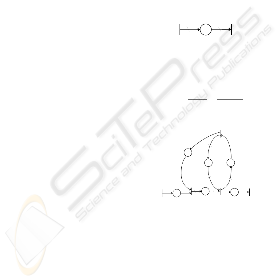
Example 1 The counter variable associated with
transition q described in Fig. 1 satisfies the follow-
ing equation:
x
q
(t) = ba
−1
(m + b x
q
0
(t − τ ))c.
b
a
t
q '
x
q
x
m
Figure 1: A simple TEGM.
Example 2 Let us consider TEGM depicted in Fig.
2. The corresponding counter variables satisfy the
following equations:
x
1
(t) = min(3 + x
3
(t − 2), u(t)),
x
2
(t) = min(b
2x
1
(t−2)
3
c, b
6+2x
3
(t−2)
3
c),
x
3
(t) = 3x
2
(t − 1),
y(t) = x
2
(t).
2
2
x
2
2
3
x
1
x
u
y
3
2
6
1
3
3
2
3
Figure 2: A TEGM.
3 DIOID, OPERATORIAL
REPRESENTATION
Let us briefly define dioid and algebraic tools needed
to handle the dynamics of TEGM’s, see (Baccelli
et al., 1992) for details.
Definition 2 (Dioid) A dioid (D, ⊕, ⊗) is a semiring
in which the addition ⊕ is idempotent (∀a, a ⊕ a =
a). Neutral elements of ⊕ and ⊗ are denoted ε and e
respectively.
ON MODELING AND CONTROL OF DISCRETE TIMED EVENT GRAPHS WITH MULTIPLIERS USING (MIN, +)
ALGEBRA
33

A dioid is commutative when the product ⊗ is com-
mutative. Symbol ⊗ is often omitted.
Due to idempotency of ⊕, a dioid can be endowed
with a natural order relation defined by a ¹ b ⇔ b =
a⊕b (the least upper bound of {a,b} is equal to a⊕b).
A dioid D is complete if every subset A of D admits
a least upper bound denoted
L
x∈A
x, and if ⊗ left
and right distributes over infinite sums.
The greatest element noted > of a complete dioid
D is equal to
L
x∈D
x. The greatest lower bound of
every subset X of a complete dioid always exists and
is noted
V
x∈X
x.
Example 3 • The set Z∪{±∞}, endowed with min
as ⊕ and usual addition as ⊗, is a complete dioid
noted
Z
min
with neutral elements ε = +∞, e = 0
and > = −∞.
• Starting from a ’scalar’ dioid D, let us consider p ×
p matrices with entries in D. The sum and product
of matrices are defined conventionally after the sum
and product of scalars in D:
(A⊕B)
ij
= A
ij
⊕B
ij
and (A⊗B)
ij
=
p
L
k=1
A
ik
⊗B
kj
.
The set of square matrices endowed with these two
operations is also a dioid denoted D
p×p
.
Counter variables associated with transitions are
also called signals by analogy with conventional sys-
tem theory. The set of signal is endowed with a kind
of module structure, called min-plus semimodule; the
two associated operations are:
• pointwise minimum of time functions to add sig-
nals:
∀t, (u ⊕ v)(t) = u(t) ⊕ v(t) = min(u(t), v(t));
• addition of a constant (∈
Z
min
) to play the role of
external product of a signal by a scalar:
∀t, ∀λ ∈ Z∪{±∞}, (λ.u)(t) = λ⊗u(t) = λ+u(t).
A modeling method based on operators is used in
(Cohen et al., 1998a), (Cohen et al., 1998b), a similar
approach is proposed here to model TEGM’s. Let us
recall the definition of operator.
Definition 3 (Operator, linear operator) An opera-
tor is a map from the set of signals to the set of sig-
nals. An operator H is linear if it preserves the min-
plus semimodule structure, i.e., for all signals u, v and
constant λ,
H(u ⊕ v) = H(u) ⊕ H(v) (additive property),
H(λ ⊗ u) = λ ⊗ H(u) (homogeneity property).
Let us introduce operators γ, δ, µ which are central
for the modeling of TEGM’s:
1. Operator γ
ν
represents a shift of ν units in
counting (ν ∈ Z ∪ {±∞}) and is defined as
γ
ν
x(t) = x(t) + ν. It verifies the following rela-
tions:
½
γ
ν
⊕ γ
ν
0
= γ
min(ν, ν
0
)
,
γ
ν
⊗ γ
ν
0
= γ
ν+ν
0
.
2. Operator δ
τ
represents a shift of τ units in
dating (τ ∈ Z ∪ {±∞}) and is defined as
δ
τ
x(t) = x(t − τ). It verifies the following rela-
tions:
½
δ
τ
⊕ δ
τ
0
= δ
max(τ, τ
0
)
,
δ
τ
⊗ δ
τ
0
= δ
τ+τ
0
.
3. Operator µ
r
represents a scaling of factor r and is
defined as µ
r
x(t) = br × x(t)c in which r ∈ Q
+
(r is equal to a ratio of elements in N). It verifies
the following relation: µ
r
⊕µ
r
0
= µ
min(r, r
0
)
. Note
that µ
r
⊗ µ
r
0
can be different from µ
(r×r
0
)
.
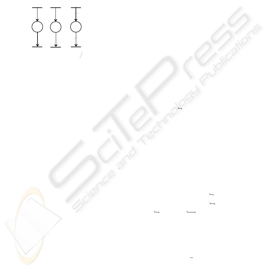
See Fig.3.a-3.c for a graphical interpretation of op-
erators γ, δ, µ respectively. We note that operators
γ, δ are linear while operator µ is only additive. We
have the following properties:
1. γ
ν
δ
τ
= δ
τ
γ
ν
, µ
r
δ
τ
= δ
τ
µ
r
(commutative proper-
ties),
2. Let a, b ∈ N, we have µ
a
−1
µ
b
= µ
(a
−1
b)
.
Let us introduce dioid D
min
[[δ]]. First, we denote
by D
min
the (noncommutative) dioid of finite sums
of operators {µ
r
, γ
ν
} endowed with pointwise min
(⊕) and composition (⊗) operations, with neutral ele-
ments ε = µ
+∞
γ
+∞
and e = µ
1
γ
0
. Thus, an ele-
ment in D
min
is a map p =
L
k
i=1
µ
r
i
γ
ν
i
such that
∀t ∈ Z, p (x(t)) = min
1≤i≤k
(br
i
(ν
i
+ x(t))c).
Operator δ is considered separately from the other
operators in order to allow the definition of a dioid of
formal power series. With each value of time delay τ
(i.e., with each operator δ
τ
) is associated an element
of D
min
. More formally, we define a map
g : Z → D
min
, τ 7→ g(τ ) in which
g(τ ) =
L
k
τ
i=1
µ
r
τ
i
γ
ν
τ
i
.
Such an application can be represented by a formal
power series in the indeterminate δ. Let the series
G(δ) associated with map g defined by:
G(δ) =
M
τ∈ Z
g(τ ) δ
τ
.
The set of these formal power series endowed with
the two following operations:
F (δ) ⊕ G(δ) : (f ⊕ g)(τ ) = f (τ ) ⊕ g(τ)
= min(f(τ ), g(τ )),
F (δ) ⊗ G(δ) : (f ⊗ g)(τ ) =
L
i∈ Z
f(i) ⊗ g(τ − i)
= inf
i∈ Z
(f(i) + g(τ − i)),
is a dioid noted D
min
[[δ]] with neutral elements
ε = µ
+∞
γ
+∞
δ
−∞
and e = µ
1
γ
0
δ
0
.
ICINCO 2004 - SIGNAL PROCESSING, SYSTEMS MODELING AND CONTROL
34
Elements of D
min
[[δ]] allow modeling the transfer
between two transitions of a TEGM. A signal x can
be also represented by a formal series of D
min
[[δ]]
(X(δ) =
L
τ∈ Z
x(τ) δ
τ
), simply due to the fact
that it is also equal to x ⊗ e (by definition of neu-
tral element e of D
min
). For example, the graph de-
picted in Fig. 1 is represented by equation X
q
(δ) =
µ
a
−1
γ
m
δ
τ
µ
b
X
q
0
(δ) where X
q
(δ) and X
q
0
(δ) denote
elements of D
min
[[δ]] associated with transitions q and
q
0
respectively.
( a ) ( c )
( b )
n
a
t
b
b a
r
=
Figure 3: Graphs corresponding to operators γ, δ, µ.
In the following, matrices or scalars with elements
in dioid D
min
[[δ]] are denoted by upper case letters,
i.e., X is a shorter notation for X(δ).
Let us extend the product notation to compose ma-
trices of operators with vectors of signals (with com-
patible dimensions). Given a matrix of operators A
and a vector of signals X with elements in D
min
[[δ]],
we set (AX)
i
def
=
L
j
A
ij
(X
j
).
Assertion 2 The counter variables of a TEGM satisfy
the following state equations:
(
X = AX ⊕ BU,
Y = CX ⊕ DU,
(2)
in which state X, input U and output Y vectors are
composed of signals, entries of matrices A, B, C, D
belong to dioid D
min
[[δ]].
Example 4 TEGM depicted in Fig. 2 admits the
following state equations:
X
1
X
2
X
3
=
ε ε γ
3
δ
2
µ
1/3
δ
2
µ
2
ε µ
1/3
γ
6
δ
2
µ
2
ε δµ
3
ε
X
1
X
2
X
3
⊕
e
ε
ε
U,
Y =
¡
ε e ε
¢
X
1
X
2
X
3
⊕ εU.
(3)
4 JUST IN TIME CONTROL
4.1 Residuation Theory
Laws ⊕ and ⊗ of a dioid are not reversible in general.
Nevertheless Residuation is a general notion in lat-
tice theory which allows defining ”pseudo-inverses”
of some isotone maps (f is isotone if a ¹ b ⇒ f (a) ¹
f(b)). Let us recall some basic results on this theory,
see (Blyth and Janowitz, 1972) for details.
Definition 4 (Residual of map) An isotone map f :
D → C in which D and C are ordered sets is residu-
ated if there exists an isotone map h : C → D such
that f ◦ h ¹ Id
C
and h ◦ f º Id
D
(Id
C
and Id
D
are
identity maps on C and D respectively). Map h, also
noted f
]
, is unique and is called the residual of map
f.
If f is residuated then ∀y ∈ C, the least upper
bound of subset {x ∈ D | f (x) ¹ y} exists and
belongs to this subset. This greatest ”subsolution” is
equal to f
]
(y).
Let D be a complete dioid and consider the isotone
map L
a
: x 7→ a ⊗ x from D into D. The greatest
solution to inequation a ⊗ x ¹ b exists and is equal to
L
]
a
(b), also noted
b
a
. Some results related to this map
and used later on are given in the following proposi-
tion.
Proposition 1 ((Baccelli et al., 1992, §4.4, 4.5.4,
4.6))
Let maps L
a
: D → D, x 7→ a ⊗ x and L
b
: D →
D, x 7→ b ⊗ x.
1. ∀a, b, x ∈ D,
L
]
ab
(x) = (L
a
◦ L
b
)
]
(x) = (L
]
b
◦ L
]
a
)(x).
More generally, if maps f : D → C and g : C → B
are residuated, then g ◦ f is also residuated and
(g ◦ f)
]
= f
]
◦ g
]
.
2. ∀a, x ∈ D, x º a x ⇔ x ¹
x
a
.
3. Let A ∈ D
n×p
, B ∈ D
n×q
,
B
A
∈ D
p×q
and (
B
A
)
ij
= ∧
n
l=1
B
lj
A
li
, 1 ≤ i ≤ p, 1 ≤ j ≤ q.
Proposition 2 The residuals of operators γ, δ, µ are
given by:
γ
ν
]
: {x(t)}
t∈Z
7→ {x(t) − ν}
t∈Z
in which ν ∈ Z ∪
{+∞},
δ
τ
]
: {x(t)}
t∈Z
7→ {x(t + τ )}
t∈Z
in which τ ∈ Z,
µ
]
r
: {x(t)}
t∈Z
7→ {d
1
r
× x(t)e}
t∈Z
in which r ∈
Q
+
(dαe stands for the superior integer part of real
number α).
Proof
Expressions of residuals of operators γ, δ are classical
(Baccelli et al., 1992, Chap. 4), (Menguy, 1997,
Chap. 4).
ON MODELING AND CONTROL OF DISCRETE TIMED EVENT GRAPHS WITH MULTIPLIERS USING (MIN, +)
ALGEBRA
35

Relatively to residuation of operator µ, let us express
that µ
r
= P µ
0
r
I in which
I : (Z ∪ {±∞})
Z
→ (R ∪ {±∞})
Z
,
{x(t)}
t∈Z
7→ {x(t)}
t∈Z
,
µ
0
r
: (R ∪ {±∞})
Z
→ (R ∪ {±∞})
Z
,
{x(t)}
t∈Z
7→ {r × x(t)}
t∈Z
and P : (R ∪ {±∞})
Z
→ (Z ∪ {±∞})
Z
,
{x(t)}
t∈Z
7→ {bx(t)c}
t∈Z
.
Operator I is residuated, its residual is defined by
I
]
: (R ∪ {±∞})
Z
→ (Z ∪ {±∞})
Z
,
{x(t)}
t∈Z
7→ {dx(t)e}
t∈Z
.
Operator P is residuated, its residual is defined by
P
]
: (Z ∪ {±∞})
Z
→ (R ∪ {±∞})
Z
,
{x(t)}
t∈Z
7→ {x(t)}
t∈Z
, we have P
]
= I.
Residuations of I and P are proven directly from
Def. 4. Indeed I, P, I
]
and P
]
are isotone, moreover,
∀t ∈ Z,
∀x ∈ (R ∪ {±∞})
Z
, I I
]
(x(t)) = I(dx(t)e) ¹ x(t)
and ∀x ∈ (Z ∪ {±∞})
Z
, I
]
I(x(t)) = dx(t)e = x(t);
∀x ∈ (Z ∪ {±∞})
Z
, P P
]
(x(t)) = P I(x(t)) =
bx(t)c = x(t) and ∀x ∈ (R∪{±∞})
Z
, P
]
P (x(t)) =
IP (x(t)) = bx(t)c º x(t).
Residual of operator µ
0
is classical, it is defined by
µ
0
r
]
: (R ∪ {±∞})
Z
→ (R ∪ {±∞})
Z
,
{x(t)}
t∈Z
7→ {
1
r
× x(t)}
t∈Z
. Hence, we can
deduce the residuation of operator µ. We have
µ
]
r
= (P µ
0
r
I)
]
= I
]
µ
0
r
]
P
]
thanks to Prop. 1.1, i.e.,
∀x ∈ (Z ∪ {±∞})
Z
, µ
]
r
x(t) = dµ
0
r
]
I(x(t))e =
d
1
r
× x(t)e.
4.2 Control Problem Statement
Let us consider a TEGM described by Eqs. (2). The
just in time control consists in firing input transitions
(u) at the latest so that the firings of output transitions
(y) occur at the latest before the desired ones. Let us
define reference input z as the counter of the desired
outputs: z
i
(t) = n means that the firing numbered
n of the output transition y
i
is desired at the latest at
time t. More formally, the just in time control noted
u
opt
is the greatest solution (with respect to the order
relation ¹) to Eqs. (2) such that y ¹ z (with respect
to the usual order relation ≤, u
opt
is the lowest control
such that y ≥ z).
Its expression is deduced from the following result
based on Residuation theory.
Proposition 3 Control u
opt
of TEGM described by
Eqs. (2) is the greatest solution (with respect to the
order relation ¹) to the following equations:
½
ξ =
ξ
A
∧
Z
C
,
U =
ξ
B
∧
Z
D
.
ξ is the greatest solution of the first equation and
corresponds to the latest firings of state transition X
(ξ º X).
Proof We deduce from Eqs. (2) that state X and
output Y are such that
½
X º AX (i)
X º BU (2i)
and
½
Y º CX
Y º DU
. Moreover, we look for control U such
that Y ¹ Z which leads to
½
Z º CX (3i)
Z º DU (4i)
.
The greatest solution to Eq. (3i) is equal to
Z
C
.
Hence we deduce thanks to Prop. 1.2 that the greatest
solution noted ξ verifying Eqs. (i) and (3i) is equal
to ξ =
ξ
A
∧
Z
C
(sizes of ξ and X are equal). So
the greatest solution verifying Eqs. (2i) and (4i) (in
which ξ replaces X) is equal to
ξ
B
∧
Z
D
.
For example let us consider the TEGM depicted in
Fig. 2 and modeled by Eqs. (3). Let us give the ex-
pression of the just in time control, which leads to cal-
culating the greatest solution of the following equa-
tions:
ξ
1
ξ
2
ξ
3
=
ξ
2
µ
(1/3)
δ
2
µ
2
ξ
3
δµ
3
∧ Z
ξ
1
γ
3
δ
2
∧
ξ
2
µ
(1/3)
γ
6
δ
2
µ
2
,
U = ξ
1
.
Let us express these equations in usual counter set-
ting. The recursive equations are backwards in time
numbering and are supposed to start at some finite
time, noted t
f
, which means that system is only con-
trolled until this time. So let us consider the following
”initial conditions”:
z(t) = z(t
f
) and ξ(t) = ξ(t
f
), ∀t > t
f
.
For all t ∈ Z , we have:
ξ
1
(t)
ξ
2
(t)
ξ
3
(t)
=
d3/2 × ξ
2
(t + 2)e
max(d1/3 × ξ
3
(t + 1)e, z(t))
max(ξ
1
(t + 2) − 3, d3/2 × ξ
2
(t + 2) − 3e)
,
u(t) = ξ
1
(t).
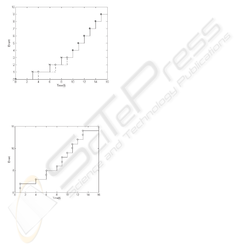
Reference input z and output y are represented in
Fig.4, z is such that z(t) = z(t
f
), ∀t > t
f
= 15.
Control u is represented in Fig.5 and is as late as pos-
sible so that desired behavior of output transition is
satisfied (y ¹ z). Moreover, control u is such that
components of ξ are greater than or equal to those of
x (x ¹ ξ).
5 CONCLUSION
Most works on dioid deal with discrete timed event
graphs without multipliers. We aim at showing here
ICINCO 2004 - SIGNAL PROCESSING, SYSTEMS MODELING AND CONTROL
36
the efficiency of dioid theory to also just in time con-
trol TEGM’s without additional difficulties. The pro-
posed method is mainly based on Residuation the-
ory and the control is the greatest solution of ”back-
ward” equations. A possible development of this
work would consist in considering hybrid systems or
more complex control objectives.
Figure 4: Output y (thin line) and reference input z (dotted
line).
Figure 5: Control u.
REFERENCES
Baccelli, F., Cohen, G., Olsder, G., and Quadrat, J.-P.
(1992). Synchronization and Linearity: An Algebra
for Discrete Event Systems. Wiley.
Blyth, T. and Janowitz, M. (1972). ”Residuation Theory”.
Pergamon Press, Oxford.
Cohen, G., Gaubert, S., and Quadrat, J.-P. (1998a). ”Al-
gebraic System Analysis of Timed Petri Nets”. pages
145-170, In: Idempotency, J. Gunawardena Ed., Col-
lection of the Isaac Newton Institute, Cambridge Uni-
versity Press. ISBN 0-521-55344-X.
Cohen, G., Gaubert, S., and Quadrat, J.-P. (1998b). ”Timed-
Event Graphs with Multipliers and Homogeneous
Min-Plus Systems”. IEEE TAC, 43(9):1296–1302.
Cohen, G., Moller, P., Quadrat, J.-P., and Viot, M. (1989).
”Algebraic Tools for the Performance Evaluation
of Discrete Event Systems”. IEEE Proceedings,
77(1):39–58.
Cottenceau, B., Hardouin, L., Boimond, J.-L., and Ferrier,
J.-L. (2001). ”Model Reference Control for Timed
Event Graphs in Dioids”. Automatica, 37:1451–1458.
Menguy, E. (1997). ”Contribution
`
a la commande des
syst
`
emes lin
´
eaires dans les dio
¨
ıdes”. PhD thesis, Uni-
versit
´
e d’Angers, Angers, France.
Munier, A. (1993). R
´
egime asymptotique optimal d’un
graphe d’
´
ev
´
enements temporis
´
e g
´
en
´
eralis
´
e : Applica-
tion
`
a un probl
`
eme d’assemblage. In RAIPO-APII,
volume 27(5), pages 487–513.
Murata, T. (1989). ”Petri Nets: Properties, Analysis and
Applications”. IEEE Proceedings, 77(4):541–580.
Nakamura, M. and Silva, M. (1999). Cycle Time Compu-
tation in Deterministically Timed Weighted Marked
Graphs. In IEEE-ETFA, pages 1037–1046.
ON MODELING AND CONTROL OF DISCRETE TIMED EVENT GRAPHS WITH MULTIPLIERS USING (MIN, +)
ALGEBRA
37
