A Comparative Study Between Neural Network and

Maximum Likelihood in the Satellite Image Classification

Antonio Gabriel Rodrigues

, Rossana Baptista Queiroz

and Arthur Tórgo

Gómez

Masters in Computer Applied, Unisinos University, Av. Unisinos 950, São Leopoldo, Rio

Grande do Sul, Brazil

Abstract. In this paper it's showed a comparative study between two tech-

niques of satellite image classification. The studied techniques are the Maxi-

mum Likelihood statistical method and an Artificial Intelligence technique

based in Neural Networks. The analyzed images were scanned by CBERS 1

satellite and supplied by Brazilian National Institute for Space Research

(INPE). These images refer to Province of Rondonia area and were obtained

by CBERS 1 IR-MSS sensor.

1 Introduction

Nowadays, one of the Remote Sensing techniques more used is the scanning of the

Earth surface by satellites. It has application in several areas, since environment

application until socioeconomic and managing applications. Some of these applica-

tions are: weather forecasting, natural resources monitoring, mapping of areas, cen-

sus systems and property registering.

The satellite image information can be extracted through classification of these im-

ages. There are various classification methods that try through several approaches to

identify with accuracy the information of each image pixel, classifying them in cate-

gories or classes according to their spectral information. Image classification meth-

ods can have different accuracy levels, according their approach and parameters

specification. Some of pixel classification methods that are more used by Geographic

Information System (GIS) are based in statistical inference. In this context it's

checked if the Artificial Intelligence based technique is suitable for image classifica-

tion.

In this paper it's presented a comparative study between two satellite image classifi-

cation techniques: the statistical method of Maximum Likelihood and an Artificial

Intelligence technique. Maximum Likelihood method is the most used in Remote

Sensing into the statistical approach. The Artificial Intelligence technique studied is

based in the use of Artificial Neural Networks [9].

Gabriel Rodrigues A., Baptista Queiroz R. and Tórgo Gómez A. (2004).

A Comparative Study Between Neural Network and Maximum Likelihood in the Satellite Image Classiﬁcation.

In Proceedings of the First International Workshop on Artiﬁcial Neural Networks: Data Preparation Techniques and Application Development, pages 1-8

DOI: 10.5220/0001130100010008

 SciTePress

The analyzed images were obtained by the China-Brazil satellite CBERS 1 (China-

Brazil Earth Resources Satellite 1) and was supplied by Brazilian National Institute

for Space Research (INPE) [9].

2 Image Classification Methods

Image classification in Remote Sensing is one of the most used techniques for ex-

tracting of information what makes possible the incorporation of this in a GIS data-

base. Classification can be understood like a space partition according to some crite-

ria [8].

Classification methods, or classifiers, can be divided in classifiers by pixel or classi-

fiers by region and can consider one or more image spectral bands (in the case of

multispectral images). Classifiers by pixel use the spectral information of each pixel

apart to find homogeneous regions defined such as classes. Classifiers by region

consider a set of neighbour pixels (region) information. This technique is also known

as contextual classification. [9] The classifiers can also be divided in supervised (in

which the classes are defined a priori based in known information) and unsupervised

(in which the classes are generated by the classifier) classifiers [2]. For the case of

the supervised classification, the classification criterion is based in the definition of

spectral signatures for each class in study obtained through training samples.

In this work it's used the classifier based in Maximum Likelihood technique that will

be explained in the next item.

2.1 Maximum Likelihood Method

Maximum Likelihood method is the most used in Remote Sensing into the statistical

approach. It's a parametrical method, once it involves parameters (mean vector and

covariance matrix) of the Multivariate Normal distribution. It's also a supervised

method because it estimates its parameters through training samples [3].

This method considers the balance of the distances among the digital level averages

of the classes through the use of statistical parameters. The distribution of the reflec-

tance values in a training area is described by a probability density function based in

Bayesan statistic. The classifier evaluates the probability of a pixel to belong a cate-

gory that it has the major probability of association [6].

Maximum Likelihood is implemented in several GISs, but the use of this classifier

presents some difficulties in the parameters estimation, specially in the covariance

matrix. Moreover, in order to produce good results it's necessary to define with a

good precision the training areas, and it requires the selection of a lot of pixels [6].

In high dimensionality data, i.e., many spectral bands information, this estimation

becomes extremely problematic due to the size of the available samples that gener-

ally in real situations it isn't sufficient.

It was noticed in some research works [1][3] that the growth of the data dimensional-

ity, (i.e., in the spectral bands number) results initially in increment in the accuracy

of the resultant classified image. It happens due to increment of the image informa-

tion available. From a certain point, however, the accuracy begins to decrease with

the same training samples due to increase of data dimensionality. This phenomena

is known like the Hughes phenomena or "the curse of dimensionality" and occurs

because with the increasing of image information is increased also the number of

parameters to be estimated, specially the covariance matrix [3].

Moreover, in Maximum Likelihood method the probability density functions of the

classes are Gaussian, approximately. McLachlan (1992, p.52) and Tou and Gonzalez

(1974, p.119) apude [2] affirms that the normal models for the probability density

functions of the classes are important in the theory as in practice, and it's suitable in

many practical applications. Haertel and Landgrebe (1999, p.2074) apude [2] say

that the distributions of the spectral classes that are present in the image generally

can be approached by the Multivariate Normal distribution, once they refers to natu-

ral scenes. The supposition of multivariate normality, however, it isn't true for all

situations and in this cases, the idea of a classifier that has a capacity to learn be-

comes appropriate, eliminating the problem of the use of a determined probabilistic

distribution [2].

2.2 Artificial Neural Networks

The conventional image classifiers used by GIS software have a difficult parameteri-

zation and in many cases they are inadequate for the needs of high accuracy de-

manded by the users [6]. In order to obtain better results and to facility the parame-

terization of these tools, it was opted to create a image classifier based in Artificial

Neural Networks.

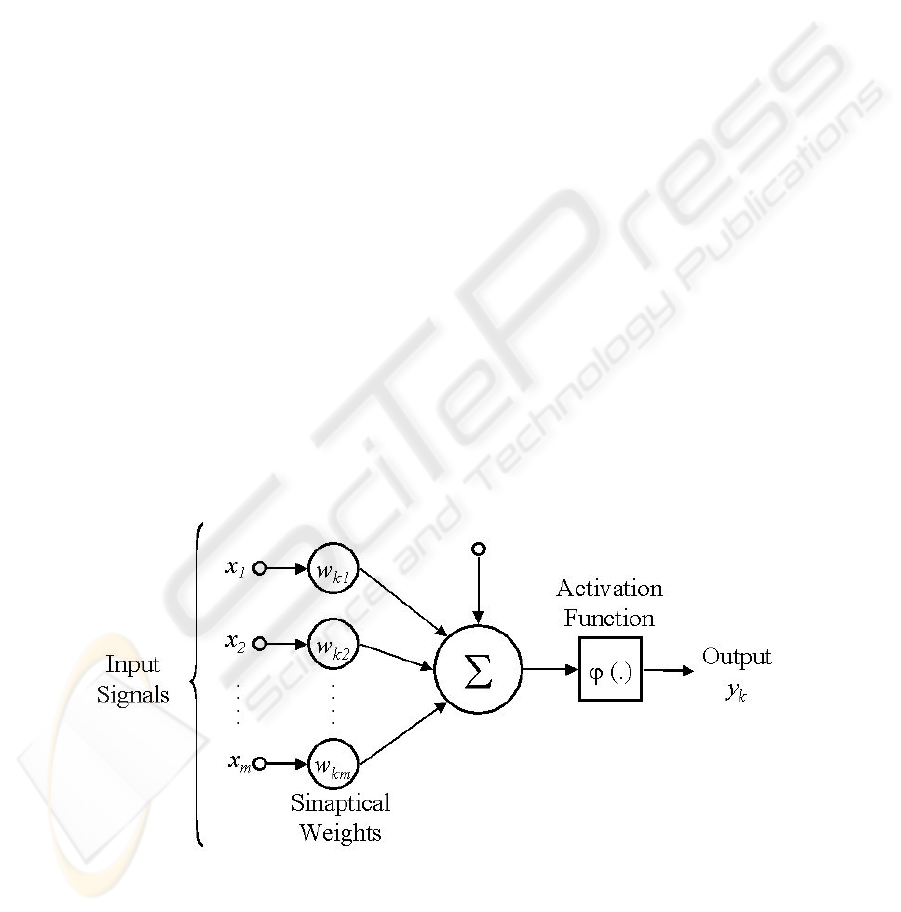
Artificial Neural Networks are algorithms whose its functioning is based in human

brain structure [2]. Its processing units are called neurons and they are formed by

three basic elements, like are illustrated in Figure 1:

Fig. 1. Neuron Model.

 a set of synapses that are connections where a signal x

in the input j and con-

nected to a neuron k are multiplied by the weight w

;

 an adder that adds the input signals, pondered by its own neuron synapses;

 a activation function that restricts the amplitude of output neuron (threshold func-

tion).

Neuronal model includes also a bias that increase or decrease the activation function

input (depending if it is positive or negative) [5].

Each input neuron receives the values of the neuron outputs connected in it. These

input signals are multiplied by its respective weights and added generating a activa-

tion value. The output value of the neuron is the result of the comparison between its

activation value and a determined score threshold defined a priori [10].

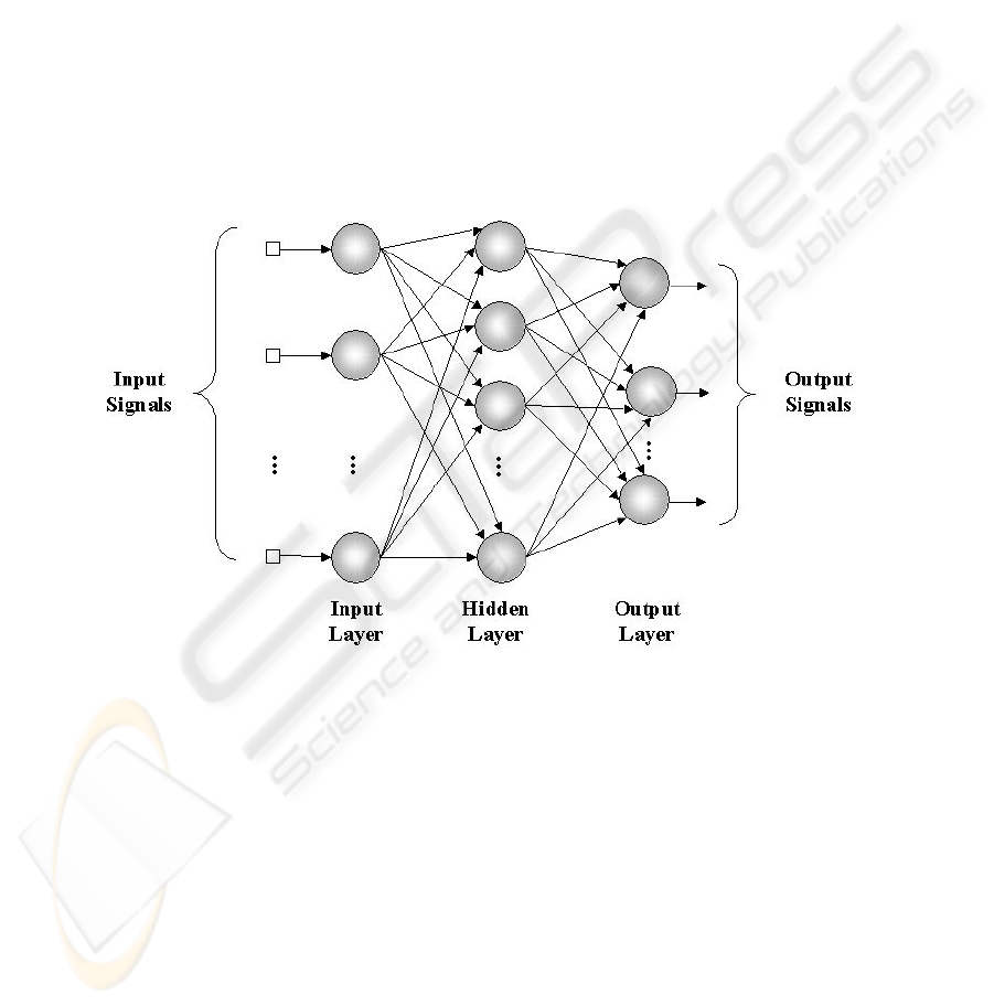
In a Neural Network the neurons are arranged in one or more layers and connected

by a great number of connections or synapses that are generally unidirectional, in

which are associate to weights in the majority of the models [2]. Its basic structure is

showed in Figure 2.

Fig. 2. Neural Network.

The capacity to learn through samples and to generalise the learned information is,

doubtless, the principal advantage of the problems solution through Neural Networks

[2]. For the learning, the networks are trained using a set of samples organized in a

set of database. During this period the synaptic weights are adjusted according to

specific mathematic proceedings that determine how the learning of the Neural Net-

works will be fulfilled. At end of this process, the acquired knowledge of the train-

ing set is represented by the set of network weights [10].

There are several types of Neural Networks models such as Recurrent Networks,

Perceptron Networks, Multi Layer Perceptron Networks, Constructive Networks, and

others [2].

The type of Neural Network that was used in this work was the Cascade Correlation

[4] that uses a supervised learning technique to train the networks. It is a Construc-

tive Network that acts on a net initially minimal (with only the input and output

layer) and introduces new intermediary units during the training, one by one accord-

ing to the need of learning. Once a new unit is added to the network, its weights are

frozen. So, this unit pass to influence the operations in the network and it is used to

detect new attributes in the set of patterns.

The unit to be included in the network can be selected from a pool of candidate units

organized as a layer. This layer is connected to the input layer and to the hidden

layers, but not in the output layer, once it should not interfere directly in the network

result. The selection of the candidate is the correlation that it has with the network

output. Therefore, the connection weight among the candidate units and the input

layers and intermediary should be defined so that it can maximize the correlation

between the candidate unit and the output layer. Thus, the candidate that to present

larger correlation will be inserted in the network as a intermediary layer and will be

connected to all the other layers [2][4].

The reason that took to opt for this network type is the fact of that is not being neces-

sary the configuration of the number of neurons of the intermediary layer, once if

Cascade Correlation is a Constructive Neural Network. This constitutes an advan-

tage, because in works that use other types of Neural Networks, just as Multilayer

BackPropagation in [10] they are necessary to do several tests with different num-

bers of neurons in the intermediary layer, in order to obtain the ideal amount of neu-

rons for better learning of the nets.

3 Experiments

To accomplish the experiments, it was used an image supplied by INPE, orbit

175/point 110 CBERS1 IR-MSS (Infra-Red Multispectral Scanner) sensor, obtained

in 2000, July, 29, that covers about 14.400 km

of the Porto Velho region in the

Province of Rondonia between 07° 50’’ and 09° 03’’ S latitudes and between the 64

10” and 62

52”O longitudes. In this image was identified and defined 4 classes:

native forest, deforestation, “no-forest” (no florestal covering area or cerrado

vegetation) and water.

To accomplish the classification it was used the Maximum Likelihood technique and

Neural Networks. To train the Neural Networks was used the NEUSIM simulator [7]

that uses the Cascade Correlation network. It was used the GIS SPRING (Sistema de

Processamento de Informações Geo-referenciadas) to make the classification with

Maximum Likelihood method.

The training and validation of the two methods was made using a set of 240 pixels

regarding the classes to be identified (60 pixels per class). Of these, was selected 120

pixels randomly that integrated the train database while the remaining 120 pixels

was used to validate the classifiers.

The training process of the Neural Network consisted in to submit the network to

learning through the sample basis that was composed of the greyscale of the spectral

bands B1, B2 and B3 to each pixel of the analysed image and also the class which

this pixel belongs. Each class are represented such as:

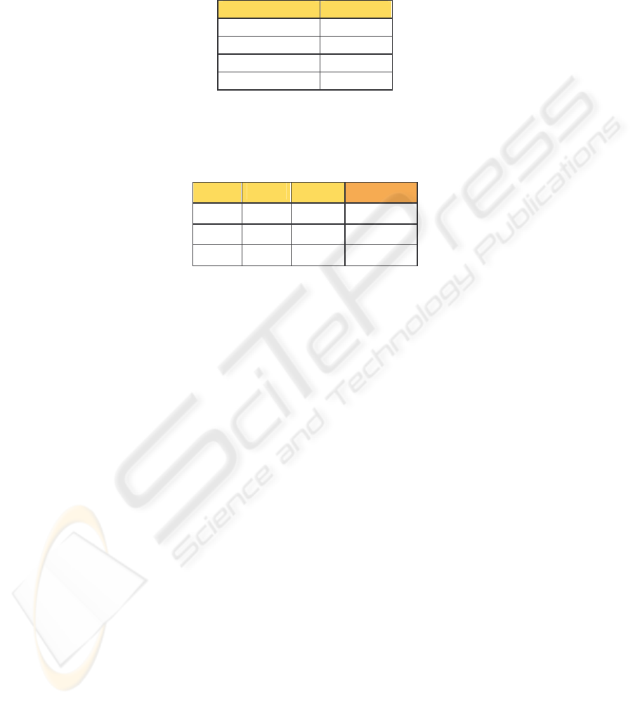
Table 1. Classes Representation.

Class Code

Deforestation

1 0 0 0

Forest 0 1 0 0

No-forest 0 0 1 0

Water 0 0 0 1

This way, the training database of the Neural Networks is organised such as showed

below:

Table 2. A Neural Network database sample.

B1 B2 B3 Class

46 33 126 0 0 0 1

57 22 89 0 1 0 0

.... .... .... ....

The Neural Network has three neurons in its input layer, each one referring to one

spectral band. The output layer has four neurons. When the input signals spread for

the network, only one of the neurons of the output layer should be activated. It was

used 10.000 epochs in the training.

The Maximum Likelihood classifier was trained with the same 120 pixels used to the

construction of de Neural Network training database.

After the training of both methods, the entire image was submitted to classification

and the results were plotted, as it will be showed in the next item.

4 Results

Starting from the accomplished experiments with the chosen techniques were gener-

ated the confusion matrix and kappa coefficient of concordance for both methods.

The confusion matrix shows how much the classifier confuses a class with other. For

this, the generated output is compared with the sample database that holds the true

results. The diagonal of the matrix shows how much the method got right, i.e., how

many pixels were classified correctly according to the true results.

The confusion matrix for both methods are showed below, represented as

the legend: (C1) Deforestation, (C2) Forest, (C3) No-forest, (C4) Water.

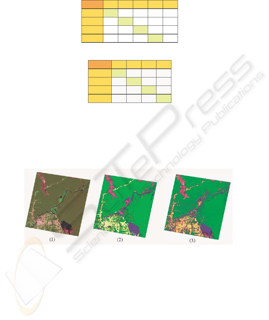
Table 3. Neural Networks confusion matrix.

Class C1 C2 C3 C4 ?

53%

17%

0% 13%

87%

13%

0% 0%

17%

13%

63%

0% 7%

0% 10%

3% 87%

Table 4. Maximum Likelihood confusion matrix.

Class C1 C2 C3 C4

30%

20%

50%

3% 87%

10%

0% 13%

87%

0% 0% 8% 92%

When the Neural Network activate more than one neuron in the output layer or when

its output approaches to zero, these results are counted in “?” column. The classifica-

tion method of Maximum Likelihood always associates one pixel to one class that it

has the major calculated probability, and so it wasn’t count undefined results.

The kappa coefficient obtained by Maximum Likelihood was 0,65 and by Neural

Networks, kappa coefficient was 0,64 in these experiments.

The results of classification of the entire image by the two methods are showed in

Figure 3.]

Fig. 3. Original Image (1) Maximum Likelihood image classified (2) Neural Networks image

classified.

Legend: Forest  No-forest Deforestation Water  ?

5 Conclusions

In the accomplished experiments, it’s noticed that both methods incline to confuse

deforestation areas with no-forests areas. It’s believed that this is due to the fact that

the reflectance values of these two classes are quite near. It’s also noticed a high

level of success in both methods for the water and native forest classes. The kappa

coefficient is considered substantial to both methods.

The classifier based in Neural Networks presented satisfactory results when com-

pared with Maximum Likelihood results, what indicates that this method is appro-

priate for satellite image classification.

References

1. Bittencourt, H. R., 2001. Reconhecimento estatístico de padrões: o caso da discriminação

logística aplicada a classificação de imagens Digitais obtidas por Sensores remotos. In

Congresso Brasileiro de Computação – CBComp 2001.

2. Braga, A. de P, Ludemir, T.B., Carvalho, A.C.P.de L.F., 2000. Redes Neurais Artificiais

Teoria e Aplicações. Livros Técnicos e Científicos Editora.

3. Erbert, M., 2001. Introdução ao Sensoriamento Remoto. Master Tesis, Universidade Fed-

eral do Rio Grande do Sul.

4. Fahlman, S. E., Lebiere, C., 1990. The Cascade-Correlation Learning Architecture. School

of Computer Science Carnegie Mellon University, Pittsburgh.

5. Haykin, S., 1999. Redes Neurais – Princípios e Prática. Bookman, 2

edition.

6. INPE, 2002.Tutorial SPRING. INPE, São José dos Campos.

7. Osório, F. S, Amy, B, 1999. A hibrid System for Constructive machine learning. Neuro-

computing, v. 28.

8. Rennó, C. D., 1998. Avaliação das Incertezas nas Classificações de Máxima

Verossimilhança e Contextual de Modas Condicionais Iterativas em Imagens Jers na

Região de Tapajós, Estado do Pará. INPE, São José dos Campos.

9. Rodrigues, A. G., Queiroz, Rossana B., Gómez, A. T., 2003. Estudo Comparativo entre os

Métodos de Classificação de Imagens de Satélite Máxima Verossimilhança Gaussiana e

Redes Neurais. In Congresso Regional de Iniciação Científica e Tecnológica em Engen-

haria – CRICTE 2003.

10.Todt, V. D., Formaggio, A. R., Shimabukuro, Y., 2003. Identificação de áreas

Desflorestadas na Amazônia através de uma Rede Neural Artificial Utilizanto Imagens

Fração Derivadas dos Dados do IR-MSS/CBERS. In XI Simpósio Brasileiro de

SensoriamentoRemoto.