
STATE OBSERVER FOR NONLINEAR SYSTEMS:
APPLICATION TO GRINDING PROCESS CONTROL
Seraphin C. Abou & Thien-My Dao
Mechanical / Manufacturing Engineering Department
Ecole de Technologie Supérieure
1100, rue Notre-Dame West
Montreal, (Quebec), H3C 1K3, Canada
Keywords: Process control; Mineral process; Nonlinear systems; Nonlinear observer; Grinding
Abstract: Due to the measurement problems encountered in mineral processes, observers are appropriate ingredients
of advanced model based control algorithm. The measurement problem can be solved by designing
nonlinear observer. This paper discusses the way in which a state observer may be designed to control a
special class of nonlinear systems. Focus is put on the pertinent applicability of the scope of these
techniques, to control the dynamics of mills in mineral processes. The approach uses a small number of
parameters to control the mill power draw affected by sudden changes within the system. It provides with
principles and ability of the system to adapt to changing circumstances due to intermittent disturbances (like
for instance changes in hardness of the raw material). Performance and stability analysis was developed.
Using a generalised similarity transformation for the error dynamics, it is shown that under boundedness
condition the proposed observer guarantees the global exponential convergence of the estimation error. This
way, the nominal performance of the process is improved but the robust stability is not guaranteed to fully
avoid the mill plugging.
1 INTRODUCTION
Grinding plants never operate at steady state but
rather at perpetual transient states due to a variety of
disturbances. The mathematical model was
addressed in the way that combines disturbance
parameters with material physical properties. It
satisfies sufficient conditions which lead to
determine the system at any instant in time.
In mineral processes, the application of modern
model based control algorithms is hampered by the
lack of accurate and cheap on-line sensors. The
design of state observers, which reconstruct states
out of a limited set of measurements, is a possible
approach for dealing with the measurement problem.
Due to the (time varying) nonlinear behaviour of
grinding systems, the measurement problem can
only be solved by designing nonlinear observers.
In general, observers design methodologies are
based on (i) exact linearisation, (ii) local
linearisation in original coordinates, (iii) local
linearisation in observer coordinates, and (iv) high
gain methods are considered (Misawa, 1989). Due to
the process uncertainty, inherent in mineral
processing, applicability and robustness analysis of
the nonlinear observers have been performed. The
stability properties analysed are with respect to zero,
which is equilibrium for the proposed system. In this
sense, our main restriction on the nominal system is
that the subsystem be globally stable with variable
viewed as a virtual control input. As a case study,
wet grinding in continuous and fed-batch operation
mode considered is described in Section 2. In
Section 3 observer design is discussed in general
while simulation results are presented in Section 4.
The observer performance analysis is discussed in
general in Section 5.
2 SYSTEM DESCRIPTION
A wet grinding shown in Fig.1 or dry grinding
(cement processing) has been developed with the
objective of studying the effects of many variables
on particle size reduction in continuous grinding
processes. Detailed phenomenological model that
describes the charge behaviour has been developed
and validated against real data (Abou, 1998).
Indeed, mineral processes present non-linear/chaotic
dynamic behaviour. Considerable efforts have been
developed in controlling such system, (Abou, 1997),
(Weller, 1980). In (Abou, 1998), a comprehensive
310
C. Abou S. and Dao T. (2004).
STATE OBSERVER FOR NONLINEAR SYSTEMS: APPLICATION TO GRINDING PROCESS CONTROL.
In Proceedings of the First International Conference on Informatics in Control, Automation and Robotics, pages 312-319
DOI: 10.5220/0001131803120319
Copyright
c
SciTePress
model integrates the physical mechanisms governing
mineral processes and a fundamental understanding
of the charge behaviour was expressed. It was
pointed out that grinding media collisions and
impacts on lifters induced non-linearity in materials
breakage process. Due to inappropriate control of
the motor charge, important engineering conclusions
derived from the charge motion studies (Abou,
1997), recommend a focused study of the influence
of the wear of both the grinding media and the lifters
on the material size reduction quality. Further
Investigation reveals that, an important factor of the
poor quality of fine grinding is due to lacks of an
appropriate control of the power draw of the mill.
This causes increase of energy consumption, and
production cost, (Austin, 1990).
To address practical results which could be
transferred to industrial level, the key is the
development of a practically an accurate grinding
circuit control. That is to maximise the
manoeuvrability at the low and the high speed
rotating stability of ball mills when the material
hardness and size or the slurry concentration change.
Figure.1: Schema of ball mill powering system
3 GRINDING PROCESS
MODELLING
Grinding systems are power-intensive, and even the
simplest ones; exhibit complex bifurcation
behaviour in going from periodic motion to chaos.
Such a complex behaviour has been noticed in the
analyses of the dynamics of the charge of ball mill
(Abou, 1998). It appears that, simple but nonlinear
models are necessary to describe such a system. The
main goal is to minimise the consumption energy,
avoid strong impact which causes wear of lifters,
and rotate the charge with optimal speed for required
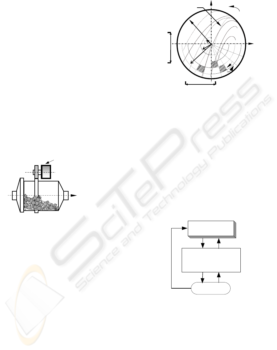
fine particle quality. Using the cross section of the
ball mill shown in Fig.1, the mill action could be
shown graphically by considering the change in
position of the centre of gravity of ball and particle
charge with increasing speed of rotation, Fig.2.
η
z
η
y
ω
ω
k <
ω
j <
ω
0
Impact
zone 1
r
j
R
ω
0
ω
j
Trajectories
of balls
ω
k
Impact
zone 2
Figure 2: Ball movement with various rotation speed
Notice that the motor load is influenced by the
filling percentage, the speed, the mill geometry and
other relevant material properties such as stiffness
and the coefficient of friction, etc… As shown in
Fig.2, theoretical position of the charge at different
rotation speed was first derived by (Davis, 1919)
based on force balance.
Most research (Austin, 1990), have developed first
order model to describe the system. However, their
use in practical solutions context has a lack of their
dependence on the physical parameters of the
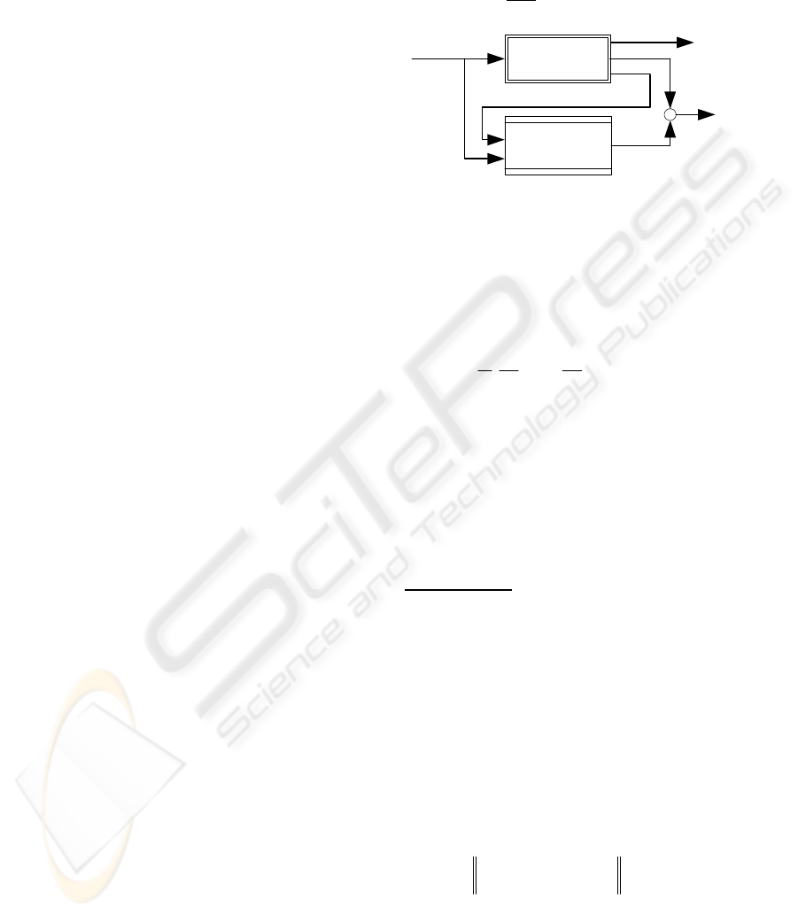
system. Since the problem is to develop the grinding
process model for control purpose, the main
objective in an advanced mathematical model
formulation could base on the following basic
control flowchart structure, Fig.3 to develop the
process behaviour.
Moto
r
Ball Mill
Definition of control
objectives
Process advanced
mathematical modelling
(,)
x
fxu
=
&
Controller
Figure 3: Control system design procedure
Notice that, besides in batch mode, grinding circuit
can operate in continuous or fed-batch mode. Based
on the interpretation of the Fig.3, we are interested
in the constitutive characteristics of the charge
motion defined by the function
(
,
)
f
xu
, focusing on
the specific parameters that better describe
continuous grinding phenomena relationship. From a
macroscopic standpoint, the internal breakage model
can be formulated taking in account the specifics
phenomena of particle transport and size reductions:
STATE OBSERVER FOR NONLINEAR SYSTEMS: APPLICATION TO GRINDING PROCESS CONTROL
311

() () ()
..
i
nn
m
.
i
x
m
tzz
∂
∂∂
∂∂∂
⎡⎤
=Ψ −Ψ⎡⎤
⎢
⎣⎦
⎣
⎥
⎦
(1)
where,
[kg], is particle mass of size i
i
m
The left side term of equation (Abou, 1998)
expresses the rate of mineral production, while the
term at the right side indicates fine particle transport
phenomena. In such a process with distributed
parameters, function Ψ
n
(.) that characterises the
particle size reduction, depends on many variables
which are absolutely linked to system performance
reliability. Therefore, without lacking for the
physical sense for the process, we can write:
(
)
(
)
.,
nn
x
uΨ=Ψ
(2)
Thus, we note the variation of the volume V of the
charge is important to the breakage mechanism as
much as it is to the transport phenomena, but from a
volumetric point of view both phenomena could be
treated in a different way. Therefore, the fraction of
the total mass broken within a tiny volume of the
charge is assumed to be
()t
σ
:
()
c
V
tad
σρ
=
∫∫∫
V
(3)
where
c
ρ
is the charge bulk density, is defined as
a mass volume of material of classes
i, so that the
flow rate of particle is:
a
()
()
c
c
VV
a
dd
dV a
dt t dt
∂ρ
σ
ρ
∂
=+
∫∫∫ ∫∫∫
dV
(4)
In worse case, where we associate to the breakage
process, the flux due to the absolute motion of the
particle, we could define the flux associate to the
fluid. However, as the mass could not be transferred
by conduction phenomena, the mass flux therefore,
vanishes, so that we could write:
i
FV
d
p
J
dF dV
dt
σ
ϑσ
=− ⋅ +
∫∫ ∫∫∫
rr
(5)
where,
i
J
r
:longitudinal diffusion flux of the mass in
class
i. ;
ϑ
:piecewise parameter;
σ
p
: local fine
particle.
Based on equation (5) for the observer design, we
assume that the mixing mechanism of powders in
ball mills can be well described by a diffusion model
and many factors such as the screen plate gape, balls
quantity and energy consumed. We deduced that, the
process could be defined as a multi-input multi-
output nonlinear system of the form:
(, ())
()
x
Fxut
ygx
=
=
&
(0)
o
x
x= (6)
where
is the state,
x∈Ω
r
uR
∈
is the control input:
m
yR∈
is the output; (0)
x
is the initial state.
It is assumed that,
∀
t the state trajectory ()
x
t is
defined. In addition, the function
(.)
F
is
continuously differentiable nonlinear function which
represents the dynamics of the process and the
disturbances.
We consider four state variables:
-
the material grinding rate,
1
()xt
-
the charge grindability,
2
()xt
-
the material fineness ,
3
()xt
-
the raw material hardness,
4
()xt
The output is set as follows:
1000
() ()
0010
yt xt
⎡⎤
=
⎢⎥
⎣⎦
(7)
Interactions of these parameters are not easily
identified.
Assumption 1. As the proposed function (.)
F
in (6)
is assumed to be C
1
, there exists a C
1
function
()x
ζ
such that
(, ())
x
Fx x
ζ
=
&
(8a)
Is globally asymptotically stable.
As result the system (6) could be designed in
parameterised nonlinear mapping form as follows:
(,,) (,,)xfxyuhxyu
=
+
&
(8b)
4 NONLINEAR OBSERVER
DESIGN
For a linear dynamical system in equation (9), a
well-known Luenburger basic linear observer theory
is given as follows:
() () ()
() ()
x
tAxtBut
y t Cx t
=
+
=
&
()
oo
x
tx
=
(9)
where
dim ; dim ; ; dim
x
n y m with n m u r
=
=>=
ˆˆ ˆ
() () () ( () ())
x
tAxtButKytCxt=++ −
&
(10)
The error dynamic equation is:
() ()et Aet=
%
&
As results, if the following conditions are satisfied:
Conditions
1.
matrix C has
rank m n<
2.
the pair
{
}
,CA
is completely observable
3.
a x transformation matrix T exists
so that
()nm−
n
K
CTAAT=−
%
4.
eigenvalues of the state matrix
A
%
have
negative real parts.
ICINCO 2004 - SIGNAL PROCESSING, SYSTEMS MODELING AND CONTROL
312
such that
(
is stable, then the state error
converges to zero. In addition we have:
)AKC−
ˆ
exx
=−
{
}
{
Re ( ) Re ( )
ji
}
A
A
αϕ
<
%
(11)
In nonlinear system as described in (6), stability
would not suffice as for Luenberger observers to
guaranty its applicability. Complete controllability is
required.
Even though the use of the nonlinear functions can
make the observer more efficient, treating the
system in the form as in (6) is a challenge. The
Jacobian matrices of
and in (6) with
respect to
x taken at α is used to design a
matrix
(,)Fxt (,)gxt
(,)t
α
Γ
which is a full rank, ( ) and
satisfies assumptions below. The system described
in (1)-(5) is highly nonlinear, clearly, it is difficult to
verify in practice assumptions that
,
and their respective time derivatives
are bounded. Therefore, there is a real incentive for
finding possible ways to lessen the complexity of the
computation of
.
n
R
α
∈
(,)/Fxt x∂∂
∂(,)/gxt x∂
1
ˆ
(,)xt
−
Γ
Therefore, by eliminating some redundant terms, we
are seeking an improvement of the proposed
observer design for a special class of the system
described in (6) using (8a) and (8b), for which
assumptions 1 hold. Proceeding by analogy to the
classical observer design approach in linear case for
SISO, it is possible to extend the high gain observer
design to MIMO cases, fig.4.
Keeping to the fact that the model described by
equations (5) and (6) are exactly the same as another
and have theoretical importance, the system could be
treated as a special class of nonlinear system when
unknown inputs are considered. In this sense, to
avoid our investigations becoming extremely
restricted circumstances where deficiencies become
apparent, we introduced the following representation
class to fairly well match the mill behaviour.
(,,)
x
Ax h x y u
yCx
=+
=
&
(12)
Equation (12) is valid for each state of the system.
The sufficient and necessary conditions that
characterise the function
may be found in
(Misawa, 1989). Therefore the following conditions
are assumed.
(,,)hxyu
Assumption 2: The observer state converges
asymptotically to the state of the system, so that the
state error is in the neighbourhood of zero.
Therefore, the unmodeled dynamics subsystems
have relative degree zero.
Assumption 3: The partial derivatives of
with respect to
(,,)hxyu
x
and their respective time
derivatives are bounded for all
x
and , so that:
u
(,,)
h
i
xyu
ij
x
j
∂
Ν=
∂
(13)
Process
Observer
u
y
e
-
+
ˆ
y
Figure 4: Nonlinear observer structure
We assumed
o
x
is an equilibrium point
corresponding to zero input and output,
i.e.,
()0;()0
oo
fx hx
=
= Functions (.) (.)
f
and h are
smooth.
We denote by
i
θ
δ
a diagonal matrix and A the
constant matrix in Brunowsky form:
2
11 1
( , ,........, )
i
k
ii i
diag
θ
δ
θ
θθ
=
(14)
01...0
001 0
0. ....
0 0 0 ....
A
i
⎡
⎤
⎢
⎥
⎢
⎥
=
⎢
⎥
⎢
⎥
⎣
⎦
(15)
The design of parameters
i
θ
δ
must be large enough
to compensate the system nonlinearity. Thus we
shall assume:
Assumptions 4:
a. Matrix (, ,)
x
yu
i
Γ
is full rank and
is defined as follow :
(,,)
(,,)
.....
1
(,,)
C
i
Cxyu
ii
xyu
i
n
Cxy
ii
u
⎡
⎤
⎢
⎥
Ψ
⎢
⎥
Γ=
⎢
⎥
⎢
⎥
−
⎢
⎥
Ψ
⎣
⎦
(16)
where
(,,) (,,)
x
yu A xyu
iiij
Ψ=+Ν
b.
There exists a positive
constant
γ
which is independent of
θ
and
satisfies condition 4. such that:
{
}
1
sup ( , , )xyu
ii i
δ
δ
γ
θθ
−
Γ
≤
&
(17)
STATE OBSERVER FOR NONLINEAR SYSTEMS: APPLICATION TO GRINDING PROCESS CONTROL
313

c.
(18)
1
1
0.0
000
(,,)
. ...
000
n
n
xyu
ϕ
ϕ
ϕ
−
⎡⎤
⎢⎥
⎢⎥
Λ=
⎢⎥
⎢⎥
⎢⎥
⎣⎦
A high gain observer design for the class of
nonlinear systems in equation (12) can be stated as
follows:
1
ˆˆˆ
() () (, , ) ( )
iii
ˆ
i
x
tAxthxyu KyCx
θ
δ
−
=+ + −
&
(19)
We define the estimation error as:
ˆ
() () ()et xt xt=−
(20)
One major problem in updating the gain of observer
in equation (19) lies in the computation of the
symbolic inverse of the matrix
(, ,)
x
yu
i
Γ . In many
cases, this may become very complicated depending
on the nonlinearities involved in the system. More
precisely, at times, the matrix
ˆ
(,,)
x
yu
i
Γ may
contain excessive number of terms and
consequently, the real time implementation of the
observer may become tedious (Iwasaki, 1999). This
in turn will bring considerable simplification to the
expression of the observer’s gain.
To this end,
(,,)
x
yu
i
Γ is consider lower triangular
and non singular for all
x
and .
u
[]
12
, , .....,
T
n
x
xx x=
(21)
Based on equation (5) to express the system
described in equation (12), the improvement of the
observer in equation (19) is related to the
simplification of the gain of the observer by
elimination of the redundant terms.
For the grinding system, it is known that the motor
load depends on the load within the mill that is
tightly related to the input feed (raw material
physical properties, tailings flow rates, energy...) and
the output (flow rate, particle distribution ...). The
evolution of the charge within the mill, (the hold-up)
reproduces some unstable behaviour and is
formulated as follows:
11 11
22 212
12
(,)
(, ,)
....................
( , ,..., , )
nn n n
xAxhxu
xAxhxxu
x
x
Ax h x x x u
=+
⎧
⎪
=+
⎪
=
⎨
⎪
⎪
=+
⎩
&
&
&
&
(22)
11
22
.......
nn
yCx
yCx
y
yCx
=
⎧
⎪
=
⎪
=
⎨
⎪
⎪
=
⎩
(23)
Based on equations (8), the function
is as
follows:
(,,)hxyu
11 1
2
212 12 2
3123 23
41234 34
(,)
(, ,)
( , , , ) exp( )
(, , , ,)
hxu xu
hxxu xx xu
hxxxu xx u
hxxxxu xx u
ε
ε
=
⎧
⎪
=+
⎪
⎨
=
⎪
⎪
=+
⎩
(24)
Based on equation (15) the matrix
(,,)
x
yu
i
Λ is
chosen such as (,,) (,,)
x
yu L xyuC
ii
Λ=
i
Similar to (, ,)
x
yu
i
Γ
we choose the
matrix (,,)Qxyu
i
as follows:
(,,)
(,,)
....
1
(,,)
C
i
CA xyu
ii
Qxyu
i
n
CA xyu
ii
⎛⎞
⎜⎟
⎜
=
⎜
⎜⎟
−
⎜⎟
⎝⎠
%
%
⎟
⎟
(25)
where
(,,) (,,)
A
xyu A xyu
iii
=+Λ
%
Further the similarity matrix transformation for the
error dynamics is:
1
(,,) (,,) (,,)
M
xyu Q xyu xyu
iii
−
=Λ
(26)
Based on the following theorem, [4.] equation (26)
is valid.
Theorem:
Assume that system (19) satisfies assumptions
a, b,
c
.
There exist
0
o
θ
> such that
o
θ
θ
∀≥ we have, for
all
ˆ
(0)
n
x
R∈
;
ˆ
(0) (0)xx
λ
−
≤ where
λ
is positive
[4.]. Therefore equation (19) becomes as follows:
11
ˆˆˆ
() () ( , , ) ( )
iiii
ˆ
i
x
tAxthxyuM KyCx
θ
δ
−−
=+ + −
&
(27)
Then the error dynamics is:
11
ˆ
() (,,) (, ,)
ˆ
(,,) (, ,)
i
ii
et Ae hxyu hxyu
ii
M
xyu Lxyu K Ce
θ
δ
−−
=+ −
⎡⎤
−+
⎣⎦
&
(28)
Note that the gain matrix
K
i
is chosen such that
matrices
A
KC
iii
−
is Hurwitz, i.e. (all the
eigenvalues of have negative real parts).
5 SIMULATION RESULTS
From the above equations the material grinding rate
within the mill,
; the charge grindability (i.e.,
total of material grinded per unity of energy),
;
the material fineness ,
and the raw material
hardness,
are presented as below.
1
()xt
2
()xt
3
()xt
4
()xt
ICINCO 2004 - SIGNAL PROCESSING, SYSTEMS MODELING AND CONTROL
314
By an easy manipulation of non linear equations we
could choose conveniently the steady-state values.
Others values are imposed from the model
(Nijmeijer, 1990). Practical problem observed on
industrial milling circuit is that, large changes of the
material feed hardness causes instability in the
system controlling. The values of the various
coefficients in the model have been tuned in such a
way that the model step responses fit with
experimental step responses. Thirteen tonnes of
material was initially loaded in the mill.
0
1 2
3 4
5
6
7
8
4
4.5
5.0
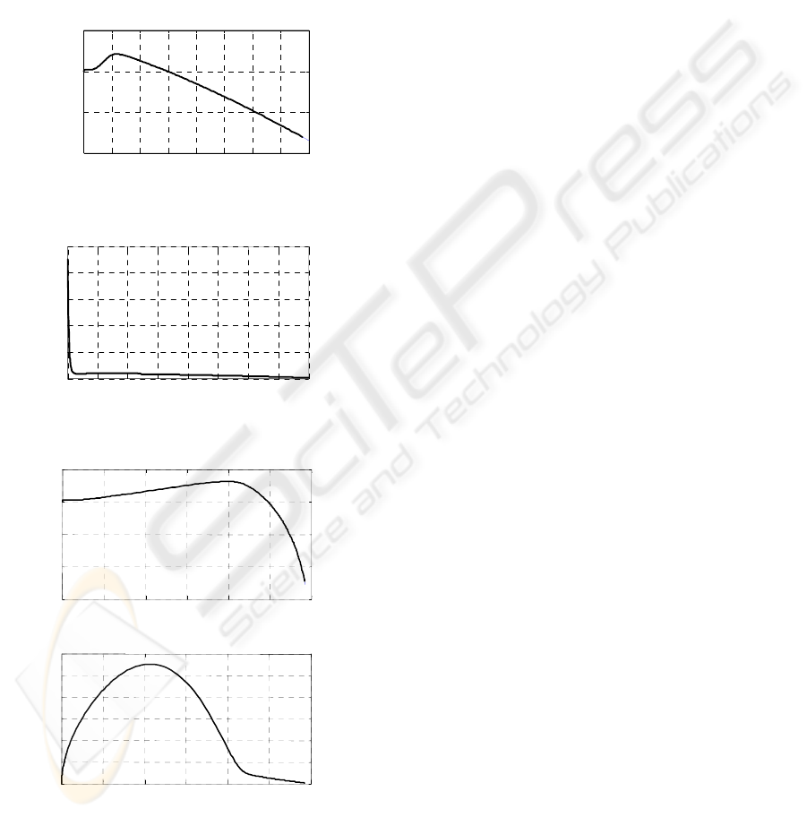
5.5
Fine particle
Time [h]
[%]
x
3
Figure 5: Percentage of fine particle
0
1 2
3
4
5
6
7
8
0
0.2
0.4
0.6
0.8
1
Material hardness
Time [h]
x
4
Figure 6: Material hardness variation
0
2
4
6
8
10
12
1
0
1
1
1
2
1
3
1
4
Rate of change of mass fraction of material
in 30x40 Mesh size fraction
Loading rate [t/h]
[t/h]
0
2
4
6
8
10
12
0
2
4
6
8
10
12
Material hold
-
up within the mill
Loading rate [t/h]
[t/h]
a
).
b)
.
Figure 7: Illustration of loading rate dependence of the
grinding performance
a)
Effect of solid flow rate on grinding rate
b)
Effect of solid flow rate on hold-up
Instead of trying to find a mathematical expression
of disturbances, a state observer in equation (27) can
be used to estimate it and compensate for it in real
time.
As a result, for the system in equations (22)-(24),
using equation (27) the estimation of the material
grinding rate,
; the charge portion that is under
going grinding per unity of input energy,
; the
material fineness ,
and the raw material
hardness,
is as follows:
1
ˆ
()xt
2
ˆ
()xt
3
ˆ
()xt
4
ˆ
()xt
1
2
3
4
ˆ
0100
ˆ
11 0 0
ˆ
ˆ
0001
ˆ
00 11
x
x
Ax
x
x
⎡
⎤
⎡⎤
⎢
⎥
⎢⎥
−
⎢
⎥
⎢⎥
=×
⎢
⎥
⎢⎥
⎢
⎥
⎢⎥
−
⎣⎦
⎣
⎦
(29)
1
2
3
4
ˆ
000
ˆ
000
ˆ
(,,)
ˆ
00 exp()0 0
ˆ
00 0 1
x
uo
x
ad
hxyu u
x
bu
x
c
ε
ε
⎡⎤
⎡
⎤⎡
⎢⎥
⎤
⎢
⎥⎢
−
⎢⎥
⎥
⎢
⎥⎢
=×
⎢⎥
⎥
+
⎢
⎥⎢
⎢⎥
⎥
⎢
⎥⎢
−
⎥
⎣
⎦⎣
⎣⎦
⎦
(30)
ˆ
i
y
yCx
=
−
%
(31)
11
22
33
44
ˆ
1000 1000
ˆ
1000 1000
ˆ
0100 0010
ˆ
0100 0010
yx
yx
y
yx
yx
⎡
⎤⎡
⎡⎤⎡⎤
⎤
⎢
⎥⎢
⎢⎥⎢⎥
⎥
⎢
⎥⎢
⎢⎥⎢⎥
=×−
⎥
×
⎢
⎥⎢
⎢⎥⎢⎥
⎥
⎢
⎥⎢
⎢⎥⎢⎥
⎣⎦⎣⎦
⎥
⎣
⎦⎣
%
⎦
i
(32)
11
ii
M
K
θ
δ
−−
ϒ=
(33)
2
1111
1
42 2
1 1 1111 12 111 1122
2
3
32 221
42
4
3 2 21 3 3 4 2 22 21 2
ˆ
1
ˆˆ ˆ
2(0.5 0.5 )
ˆˆ
exp( ) 1
ˆˆ
(2 ) 2 ( )
xku
x
xkxxxkk
xx u k
xkxxxkk
θε
θθθ
εθ
θθθ
⎡
⎤
−++ +
ϒ
⎡⎤
⎢
⎥
⎢⎥
−++ −++
ϒ
⎢
⎥
⎢⎥
=
⎢
⎥
⎢⎥
ϒ
−+ ++
⎢
⎥
⎢⎥
⎢
⎥
ϒ
⎣⎦
−+ − + +
⎣
⎦
(34)
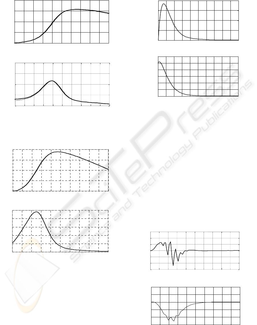
In figures 8, 9 are shown the simulation results for
the observer and the system, while the tracking error
is shown in fig.10, 11.
STATE OBSERVER FOR NONLINEAR SYSTEMS: APPLICATION TO GRINDING PROCESS CONTROL
315
0
0.5
1
1.5
2
2.5
3
3.5
4
4.5
5
0
2
4
6
8
Rate of change of mass fraction x1
(
solid: s
y
stem
)
;
(
dashed: observer
)
tim e [h]
Grinding
rate [t/
h]
0
0.5
1
1.5
2
2.5
3
3.5
4
4.5
5
0.05
0.1
0.15
0.2
0.25
Grindability x2
(solid: system ); (dashed: observer)
tim e [h]
[t/Kwh]
a.)
b.)
Figure 8: Output response of the system and the observer
a.)
Rate of change of mass fraction
b.)
Grindability
0
0.5
1
1.5
2
2.5
3
3.5
4
4.5 5
0
5
10
15
20
Percentage of fine particle x3,
(solid: system); (dashed: observer)
time [h]
[%]
0
0.5
1
1.5
2
2.5
3
3.5
4
4.5 5
0
0.2
0.4
0.6
0.8
1
Material hardness x4,
(solid: system); (dashed: observer)
time [h]
a.)
b
.
)
Figure 9: Output response of the system and the observer
a.)
Percentage of fine particle
b.) Material hardness
0
0.5
1
1.5
2
2.5
3
3.5
4
4.5
5
0
0.01
0.02
0.03
0.04
Tracking error for the rate of change
x1-x1es
time [h]
[t/h]
0
0.5
1
1.5
2
2.5
3
3.5
4
4.5
5
0
0.02
0.04
0.06
0.08
0.1
0.12
Tracking error for grindability x2-x2es
time [h]
[t/Kwh]
Figure 10: Grindability and rate of change tracking error
6 ROBUSTNESS AGAINST
STRUCTURAL UNCERTAINTY
In practice, from the test results, correlation for
samples could not be obtained because of different
geological origins. However, experimental
relationships between dynamic elastic parameters
and Bond grindability, (Van Heerden, 1987), were
used to valid the observer simulation results. In the
dynamical analysis the dynamics of the error system,
obtained by combining the experimental process
results with the observer designed is analysed.
Fig.12 shows that the observer is stable for unknown
input.
0
0.5
1
1.5
2
2.5
3
3.5
4
4.5
5
-1.5
-1.0
-0.5
0
0.5
1.0
1.5
x 10
-
4
Tracking error for fine particle x3-x3es
time [h]
[%]
0
0.5
1
1.5
2
2.5
3
3.5
4
4.5
5
-3
-2
-1
0
1
2
x 10
-
4
Tracking error for material hardness x4-x4es
time [h]
Figure 11: Fine particle percentage and material hardness
tracking error
ICINCO 2004 - SIGNAL PROCESSING, SYSTEMS MODELING AND CONTROL
316

Grinding rate [t/h]
0
0.5
1
1.5
2
2.5
3
3.5
4
4.5
5
0
1
2
3
4
5
6
Rate of change of mass fraction x1, (solid: system);
(dashed: observer)
Figure 12: Observer convergence for unknown input
7 DISCUSSION
As a case study of mineral processing, the wet
grinding ball mill operated in continuous or fed-
batched mode has been studied. Simulation results
showed that significant part of the steady state error
is due to the model part and thus independent of the
observer design methodology. The robustness
against parametric and structural uncertainty can be
increased, although this will increase the noise
sensitivity. Since we herein want to track only the
truly time-varying features of the process dynamics,
the state observer designed strategy is satisfactory.
The load within the mill should be controlled at a
well chosen level because too high levels of the load
in the mill create process disturbances. The output
product fineness depends on the solids rate flow. In
view of the approximations involved in this
treatment, the agreement between the observer and
the model is remarkable. The estimation of the
observer converges to zero exponentially.
8 CONCLUSION
We have described symbolic computations for
reducing a nonlinear system to observable forms.
These tools can be applied to systems that are
linearly observable, locally observable with zero
input or merely locally observable.
The key impact of this development lies in the
system ability, to reduce material residence time, to
flow information and material in a much-improved
manner with the appropriate control strategy.
Additional elements to be considered in the
evaluation of the performance of the observer are
distributed parameters effects due to the large
sampling intervals often encountered in mineral
applications.
REFERENCES
Abou S.C., 1998. Contribution to ball mill modelling ‘’.
Doctorate thesis, Laval University, Ca,
Abou S.C., 1997. Grinding process modelling for
automatic control: application to mineral and cement
industries‘’. Engineering Foundation Conferences,
Delft, the Netherlands
Austin L. G., 1990. A mill power equation for SAG mills.
Minerals and Metallurgical Processing, pp.57-62.
Busawon K. ,Ratza M.& Hammouri H, 1998. Observer
design for a class of nonlinear systems. Int. J. Control
71, pp.405-418.
Davis, E.W., 1919. Fine crushing in ball mills. AIME
Transaction, vol. 61, pp.250-296.
Iwasaki M., Shibata, & Matsui., 1999. Disturbance-
observer-based nonlinear friction compensation in
table drive system. IEEE/ASME Trans. Mechatronic,
vol.4. pp.3-8.
Misawa E.A. & Hedrick J.K., 1989. Nonlinear observer. A
state of the art survey,. Trans. of the ASME, 111,
pp.344-352.
Morell S., 1993. The prediction of powder draw in wet
tumbling mills. Doctorate thesis, University of
Queensland.
Nijmeijer, H., & Van Der Schaft A.J., 1990. Nonlinear
dynamical control systems”. Springer Berlin.
Plummer A.R. & Vaughan N.D., 1996. Robust adaptive
control for Hydraulic Servo-systems, ASME J. of
dynamic systems, Measurement, and control. No 11.,
pp.237-244
Van Heerden, W.L., 1987. General relations between static
and dynamic moduli of rocks, (pp. 381-385). Int. J.
Rock Mech. Min. Sci. Geomech. no. 24.
Weller K. R, 1980. Automation in mining, mineral and
metal processing, Proc. 3rd IFAC symposium
Pergamon Press
. pp. 295-302
STATE OBSERVER FOR NONLINEAR SYSTEMS: APPLICATION TO GRINDING PROCESS CONTROL
317
