FUZZY CONTROLLER DESIGN FOR A THREE JOINT ROBOT

LEG IN PROTRACTION PHASE

An optimal behavior inspired fuzzy controller design

Mustafa Suphi Erden, Kemal Leblebicioğlu

Department of Electrical & Electronics Engineering, Computer Vision and Intelligent Systems Research Laboratory,

Middle East Technical University, 06531 Ankara, Turkey

Keywords: Robot leg, fuzzy controller, optimal control.

Abstract: A fuzzy controller design is performed for a three joint robot leg in protraction phase. The aim is to develop

a controller to carry the tip point to any given destination. The design is based on the inspirations derived

from optimal behaviors of the leg. The optimal trajectories are obtained by using optimization methods

utilizing “numerical gradient” and “optimal control” successively. Separate fuzzy controllers are designed

for each actuator. In writing the rules each actuator is considered to be an independent agent of the leg

system. The protraction motion is divided into two epochs. For each epoch different controller systems are

designed to switch from one to the other in between.

1 INTRODUCTION

The aim in this study is to design a fuzzy controller

system, which will carry a three joint robot leg from

any initial position to any commanded position in a

protraction phase. In Fig.1 a schematic

representation of a three joint robot leg is given. A

three joint robot leg can be considered as a three

joint robot manipulator. Eq.1 relates the tip point

position to the three joint angles. In this equation

)(

, represents the position of the tip point with

respect to the body frame, when the joint angles take

the values in the

vector. The variables in the form

of a

represent the length of the ith link. The

variables in the form of

mean the sum of the ith

and jth joint angles (

). The variables in the

form of c

are not shown in the figure but exist in the

equation. (-c

,0,0) represents the position of the

center of gravity of the ith link with respect to the ith

coordinate frame. Namely, the term (a

-c

) designates

the distance of the center of gravity of the ith link

from the ith joint.

In order to calculate the energy dissipated in

actuators during a protraction phase, one needs to

calculate the joint torques throughout the movement.

* This research is supported by the research fund

of Middle East Technical University as a scientific

research project: BAP – 2002 – 03 – 01 – 06.

If the motion is slow, the inertial related forces

due to acceleration, Coriolis and centrifugal effects

can be neglected and the torque can be calculated as

resulting only by the gravitational forces. Namely, if

the motion is slow, the result of a static analysis of

torques can be substituted for the dynamic analysis.

This means that the torques are equal in amount and

direction to compensate the gravitational force on

the leg. In Eq.2, the torque vector (Q

, Q

) for a

position represented by the

vector is given. The

, m

values in this equation correspond to the

link masses, and g is the gravitational acceleration.

(1)

(2)

Figure 1: A three joint leg diagram with coordinate

frames attached to the links.

302

Suphi Erden M. and Leblebicio

glu K. (2004).

FUZZY CONTROLLER DESIGN FOR A THREE JOINT ROBOT LEG IN PROTRACTION PHASE - An optimal behavior inspired fuzzy controller design.

In Proceedings of the First International Conference on Informatics in Control, Automation and Robotics, pages 302-306

DOI: 10.5220/0001132503020306

 SciTePress

In robotic applications it is common to use the

sum of squares of joint torques as a criteria of

dissipated energy (Bobrow et al., 2001; Liu et al.,

2000). Following this approach, Eq.3 will be utilized

as a criterion of dissipated energy in this study. The

input of the three joint leg system for a protraction

movement is the trace of joint velocities throughout

the protraction period. This period is taken to be 5

seconds in this work. The input vector at a time

instant can be represented as in Eq.4.

2 TRAJECTORY OPTIMIZATION

The energy optimization problem for the protraction

movement of three joint leg can be stated as to find

the optimal

)(tu trajectory to minimize Eq.3 from

the initial to the final time with given initial and

final tip point positions. This problem is a typical

“optimal control” problem, which is trivial to

formulate and solve (see, e.g. Kirk, 1970). However,

the solution of this optimal control problem is very

much dependent on the initial trajectory used at the

start. If the initial trajectory is not feasible, it is very

probable that the resultant trajectory will also not be

feasible. Therefore, the optimal control technique

needs a feasible initial trajectory. In order to

generate this initial trajectory a method using

“numerical gradient”, in which feasibility is imposed

by penalty functions, is used. The output trajectories

of this method were pretty good. The optimal control

method then is used to tune the trajectories slightly

around the trajectories found by the initial method.

In the method based on the numerical gradient

the conventional method of “steepest descent” is

utilized after the problem is discretized. The total

duration is divided into 50 equal durations, and the

starts of durations are signified as the 50 time

instants (denoted by n). The actuators are assigned a

velocity at each instant and this velocity is held

constant in the sub-period starting with that instant.

In this way, the movement of an actuator is

accomplished by 50 velocity values throughout the

protraction period of 5 seconds. Since there are three

actuators, the input vector which makes the system

to accomplish a whole protraction is a 50

3 long

vector ( ). The initial and final tip point positions

are constant. Therefore the required joint angles for

initial and final positions are given. Initial input,

namely initial trajectory of joint velocities, is taken

as the average velocity that would take the tip point

from the initial position to the final. The cost

function is constructed by summing up the following

four penalty functions. Eq.5 is the penalty related

with the sum of torque squares. Eq.6 is the penalty

to avoid the tip point of the leg to go under the

ground (ground level is –5). Eq.7 is the penalty

function related with the joint angle limits. The last

penalty in Eq.8 is related with the required final

condition of angles. If the final angles are not equal

to the required values this term becomes positive.

The overall cost function (Eq.9) is a weighted

sum of these four penalties. The values of these

weights are taken as follows: T=1; U=200; R=0.01;

F=1000. These values are arranged by trial and error

in order to make the four costs comparable and to

force the algorithm to generate some feasible

solution. According to the steepest descent

algorithm, the gradient of the cost function with

respect to the input vector is found and the input

vector is iterated in the opposite direction of the

gradient. The value of

in Eq.10 is determined by a

one-dimensional search in each iteration.

In order to determine the trajectories with the

optimal control technique, first the Hamiltonian

formulation of the problem should be performed,

and then the differential equations should be

numerically solved. Following the notation in (Kirk,

1970), the Hamiltonian formulation, necessary

conditions and boundary conditions for the three

joint leg problem are given in Eq.9, 10, and 11,

respectively. The first two equations of the

necessary conditions make up two differential

equations whose initial and final conditions are

given respectively by the boundary conditions

equations. Starting with an initial

)(tu trajectory

these equations can be solved numerically. Next the

)(tu trajectory can be updated in the direction to

minimize the third equation of necessary conditions.

After some iteration the optimal

)(

trajectory,

which makes the third necessary condition as close

as possible to 0, can be achieved. This technique is

called “the method of steepest descent for two-point

boundary-value problems” (Kirk, 1970). The initial

)(tu trajectory for this technique is taken from the

[

]

n,j

FUZZY CONTROLLER DESIGN FOR A THREE JOINT ROBOT LEG IN PROTRACTION PHASE - AN OPTIMAL

BEHAVIOR INSPIRED FUZZY CONTROLLER DESIGN

303

output of the initial method and it is further

improved by the optimal control method.

Hamiltonian formulation

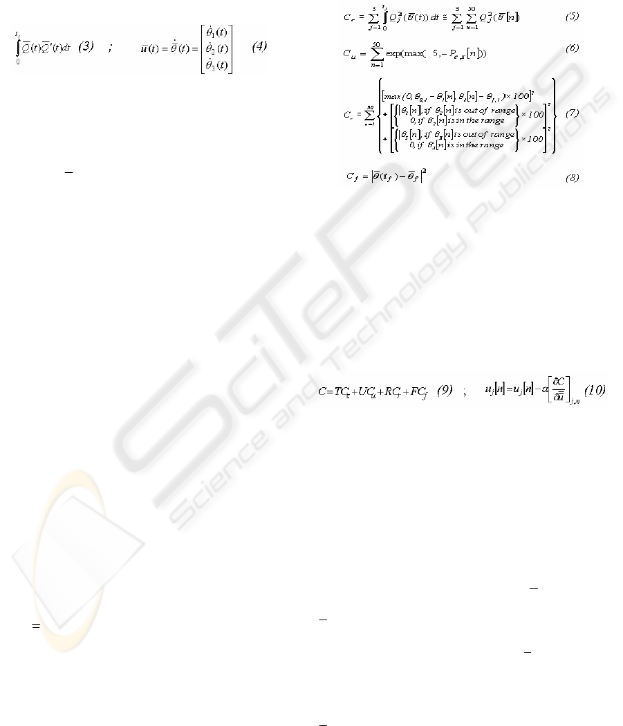
(9)

Necessaryconditions (10)

BoundaryConditions (11)

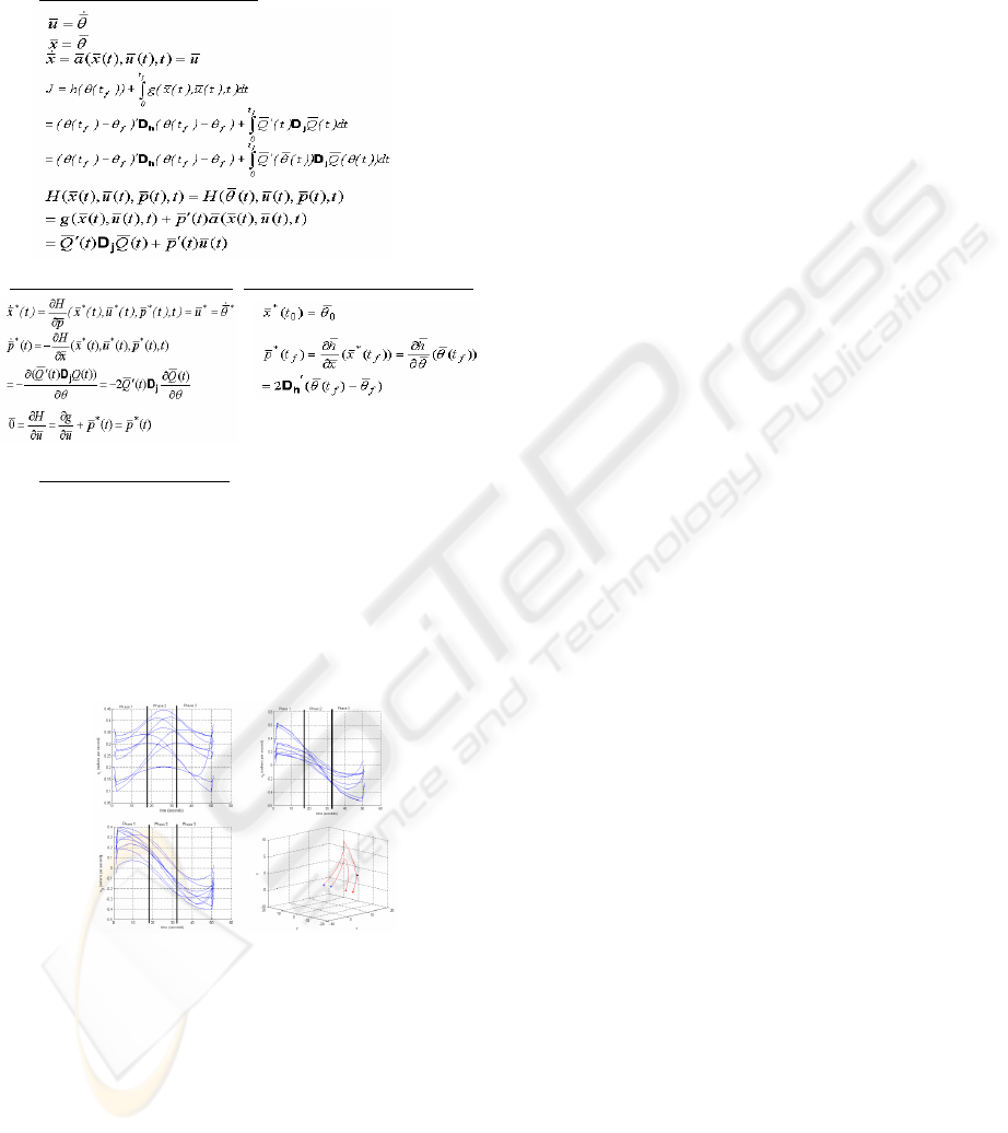
Optimization Results:

The optimization is performed for nine pairs of

initial and final tip point positions. In Fig.2, the first

three figures respectively show the three joint angle

velocities of the nine results. The fourth figure

shows the tip point trajectories for two of those nine

results. The fuzzy controller design will be

accomplished with the intuitive feeling derived from

these four figures.

3 FUZZY CONTROLLER

In order to get an intuitive feeling of the behavior of

actuators, the optimal velocity trajectories are

separated into three phases (Fig.2, first three

figures), with straight tick lines. The first phase

corresponds to the ascending of the tip point, the

second phase corresponds to the period during

which the tip point is at highest levels, and the third

phase corresponds to the descending of the tip point

towards the destination. These three phases are

possible to be distinguished by the value of the first

actuator angle. Roughly, it can be stated that, the

center of the first phase is the time when the first

joint angle is

/4 radians, the center of the second

phase is when the first joint angle is

/2 radians,

and the center of the third phase is when the first

joint angle is 3

/4 radians. In the first phase the first

angle, which is most effective for furthering the tip

point in the y direction, moves with a rather slow

velocity (Fig.2, first figure). It makes its peak in the

second phase and stays close to that maximum

value. In the third phase the velocity decreases to

lower values gradually. Roughly we can state that,

the first angle moves very slow in the first and third

phases and moves with a constant high velocity in

the second phase. The behaviors of the second and

third angles are very similar (Fig.2, second and third

figures). In the first phase they have positive big

velocities, in the second phase they have small

velocities around zero, and in the third phase they

have negative big velocities. Roughly we can state,

the second and third angles move with constant

positive and negative high velocities in the first and

third phases respectively, and they stay stationary in

the second phase. These intuitive feelings will be

useful in writing the rules for the controller of each

angle.

The whole motion is controlled with two

different controller systems each of which has

different controllers for the three joint angles. The

whole motion can be roughly divided into two

epochs of ascending and descending. The ascending

epoch corresponds to the first phase and first half of

the second phase. The descending epoch

corresponds to the last half of the second phase and

the third phase. The boundary between these two

epochs is roughly the instant at which the first angle

/2 radians. The first controller will make the tip

point rise according to the behaviors of the angles in

the corresponding phases, and the second controller

will bring the tip point to its destination again

according to the behaviors in the corresponding

phases. Moreover, the second controller has to

satisfy the stability around the destination point at

the end of the second epoch. In fact this is the

crucial point which explains the need of different

controller systems for ascending and descending..

In (Erden et al., 2004) we had developed a multi

agent perspective based fuzzy controller design

paradigm for robot manipulators. The idea there was

Figure 2: Optimal joint angle velocities for nine results

and tip point trajectories for two results

ICINCO 2004 - ROBOTICS AND AUTOMATION

304

to consider every actuator as an independent agent

and to design a fuzzy controller for every actuator.

In designing the fuzzy controller for an agent

(actuator), the infinitesimal movement of the tip

point resulting from the movement of the actuator is

considered. In other words, in constructing the rule

for an agent at any instant, all the other agents

(actuators) are considered to be stationary. The rule

is constructed in a way that the agent will make the

best action in order to make the tip point move in the

desired direction. The same idea is utilized here in

developing the rules for the fuzzy controllers of

actuators in both of the two controller systems.

In the first epoch there are the first and second

phases. These phases will be distinguished by the

value of the first actuator angle. The value S (small)

for the first actuator angle (θ

) will correspond to the

first phase and M (medium) will correspond the

second phase. The aim in this epoch is to rise up the

tip point; therefore the second input of the

controllers will be the height information, namely

the z value of the tip point (dz). The exact

membership functions and rule tables will not be

given here due to the lack of space. In the second

epoch the aim is to carry the tip point to its final

position, and to make the tip point stay there in a

stable manner. In order to accomplish these

following steps are performed: (

1) The rules that will

carry the tip point from any initial position to any final

position as if it should follow a straight-line path are

written. (2) The rules that will stop the tip point at the

final position are added.

With these ideas, first a

controller that carries the tip point to any given

destination is designed. Then the stability is satisfied

at the destination point. Without this second step, the

tip point would not have a good steady state

behavior around the final position; it would be

tending to make small circles. With these two steps a

controller which carries the tip point to any

destination and which stops it there is obtained.

In constructing the rules the following three

items are considered:

1.The first actuator will take care of the position

difference in the y direction.

2.The second and third actuators will take care of the

position difference in x and z directions, and they will

behave as if they are in a vertical plane in every instant.

3.The first actuator will take care of the behaviors

associated with the second and third phases. Namely, the

first actuator will be fast in the second phase and slow in

the third phase.

To clarify the idea in the second item here will

be given an example. The input to the second and

third actuators are the angles of the second and third

actuators (state information of the agents) and the

position differences in x and z directions. For the

state information of the second agent (for the second

joint angle, θ

) there are three membership

functions: S (small,

/4 radians), M (medium,

radians), and B (big, 3

/4 radians). For the state of

the third agent (θ

) the three levels take negative

values: NS (-

/4), NM (-

/2), and NB (-3

/4). The

example here is for the state of θ

:M; θ

:NS. Fig.3

shows the graphical representation, assuming that

the leg is in a vertical plane. Examining Fig.3, the

following statements can be derived:

1.When θ

:M and θ

:NS, a positive change in θ

will

result in a small negative change in x direction.

2. When θ

:M and θ

:NS, a positive change in θ

will

result in a medium positive change in y direction.

3. When θ

:M and θ

:NS, a positive change in θ

will

result in no change in x direction.

4. When θ

:M and θ

:NS, a positive change in θ

will

result in a big positive change in y direction.

The total amount of action to change the y

position of the tip point will be determined by the

position difference in the y direction between the tip

point and destination. Then this work will be divided

between the agents. In order to change the y

position, agent

should take a small portion and

agent

should take a bigger portion of workload. The

same logic will apply for the x direction. In order to

change the x position, agent

should take full load of

work and agent

should not have any contribution.

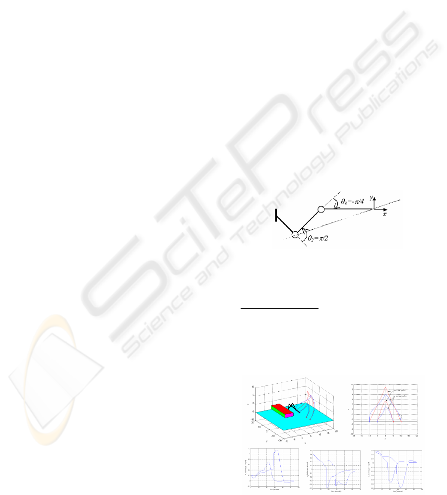
Simulation Results:

In Fig.4 the results obtained using the control

system are shown. As it is seen in the upper two

figures the controller is successful to produce tip

point trajectories ‘resembling’ the optimal ones. The

three figures below show the three joint velocity

trajectories.

Figure 3: Graphical representation of the situation

when θ

:M and θ

:S.

Figure 4: Simulation results.

FUZZY CONTROLLER DESIGN FOR A THREE JOINT ROBOT LEG IN PROTRACTION PHASE - AN OPTIMAL

BEHAVIOR INSPIRED FUZZY CONTROLLER DESIGN

305

REFERENCES

Bobrow, J.E., Martin, B., Sohl, G., Wang, E.C., Park, F.C,

Kim, K., 2001. Optimal robot motions for physical

criteria, Journal of Robotic Systems, 18(12):785-792.

Erden, M.S., Leblebicioğlu, K. and Halıcı, U., 2004.

Multi-agent system based fuzzy controller design with

genetic tuning for a service mobile manipulator robot

in the hand-over task, Journal of Intelligent and

Robotic Systems, 38: 287-306.

Kirk, Donald E, 1970. Optimal Control Theory – An

Introduction, Prentice-Hall Inc., Englewood Cliffs,

New Jersey.

Liu, J.F., Abdel-Malek, K., 2000. Robust control of planar

dual-arm cooperative manipulators, Robotics and

Computer-Integrated Manufacturing, Vol.16, No. 2-3:

109-120.

ICINCO 2004 - ROBOTICS AND AUTOMATION

306