
FUZZY MODEL BASED CONTROL APPLIED TO IMAGE-BASED
VISUAL SERVOING
Paulo J. Sequeira Gonc¸alves
Escola Superior de Tecnologia de Castelo Branco
Av. Empres
´
ario, 6000-767 Castelo Branco, Portugal
L.F. Mendonc¸a, J. M. Sousa, J. R. Caldas Pinto
Technical University of Lisbon, IDMEC / IST
Av. Rovisco Pais, 1049-001 Lisboa, Portugal
Keywords:
visual servoing, robotic manipulators, inverse fuzzy control, fuzzy compensation, fuzzy modeling.
Abstract:
A new approach to eye-in-hand image-based visual servoing based on fuzzy modeling and control is proposed
in this paper. Fuzzy modeling is applied to obtain an inverse model of the mapping between image features
velocities and joints velocities, avoiding the necessity of inverting the Jacobian. An inverse model is identified
for each trajectory using measurements data of a robotic manipulator, and it is directly used as a controller.
As the inversion is not exact, steady-state errors must be compensated. This paper proposes the use of a
fuzzy compensator to deal with this problem. The control scheme contains an inverse fuzzy model and a
fuzzy compensator, which are applied to a robotic manipulator performing visual servoing, for a given profile
of image features velocities. The obtained results show the effectiveness of the proposed control scheme:
the fuzzy controller can follow a point-to-point pre-defined trajectory faster (or smoother) than the classic
approach.
1 INTRODUCTION
In eye-in-hand image-based visual servoing, the Jaco-
bian plays a decisive role in the convergence of the
control, due to its analytical model dependency on
the selected image features. Moreover, the Jacobian
must be inverted on-line, at each iteration of the con-
trol scheme. Nowadays, the research community tries
to find the right image features to obtain a diagonal
Jacobian (Tahri and Chaumette, 2003). The obtained
results only guarantee the decoupling from the posi-
tion and the orientation of the velocity screw. This
is still a hot research topic, as stated very recently in
(Tahri and Chaumette, 2003).
In this paper, the previous related problems in the
Jacobian are addressed using fuzzy techniques, to ob-
tain a controller capable to control the system. First, a
fuzzy model to derive the inverse model of the robot is
used to compute the joints and end-effector velocities
in a straightforward manner. Second, the control ac-
tion obtained from the inverse model is compensated
to nullify a possible steady-state error by using a fuzzy
compensation.
A two degrees of freedom planar robotic manipu-
lator is controlled, based on eye-in-hand image-based
visual servoing using fuzzy control systems.
The paper is organized as follows. Section 2 de-
scribes briefly the concept of image-based visual ser-
voing. The problem statement for the control prob-
lem tackled in this paper is presented in Section 3.
Section 4 presents fuzzy modeling and identifica-
tion. Fuzzy compensation of steady-state errors is de-
scribed in Section 5. Section 6 presents the experi-
mental setup. The obtained results are presented in
Section 7. Finally, Section 8 present the conclusions
and the possible future research.
2 IMAGE-BASED VISUAL
SERVOING
In image-based visual servoing (Hutchinson et al.,
1996), the controlled variables are the image features,
extracted from the image containing the object. The
choice of different image features induces different
control laws, and its number depends also on the num-
ber of degrees of freedom (DOF) of the robotic ma-
nipulator under control. The robotic manipulator used
as test-bed in this paper is depicted in Fig. 1, and it has
2 DOF. Thus, only two features are needed to perform
the control. The image features, s, used are the coor-
dinates x and y of one image point.
143
Sequeira Gonçalves P., Mendonça L., Sousa J. and Caldas Pinto J. (2004).
FUZZY MODEL BASED CONTROL APPLIED TO IMAGE-BASED VISUAL SERVOING.
In Proceedings of the First International Conference on Informatics in Control, Automation and Robotics, pages 143-150
DOI: 10.5220/0001133201430150
Copyright
c
SciTePress

Z
0
X
0
Y
0
q
1
-q
2
Z
c
X
c
Y
c
Figure 1: Planar robotic manipulator with eye-in-hand,
camera looking down, with joint coordinates, and world and
camera frames.
2.1 Modeling the Image-Based
Visual Servoing System
In this paper, the image-based visual servoing sys-
tem used is the eye-in-hand system, where the camera
is fixed at the robotic manipulator end-effector. The
kinematic modeling of the transformation between
the image features velocities and the joints velocities
is defined as follows. Let
e
P be the pose of the end-
effector (translation and rotation), and
c
P be the pose
of the camera. Both depend on the robot joint vari-
ables q. Thus, the transformation from the camera
velocities and the end-effector velocities (Gonc¸alves
and Pinto, 2003a) is given by:
c
˙
P =
c
W
e
·
e
˙
P, (1)
where
c
W
e
=
c
R
e
S (
c
t
e
) ·
c
R
e
0
3×3
c
R
e
(2)
and S(
c
t
e
), is the skew-symmetric matrix associated
with the translation vector
c
t
e
, and
c
R
e
is the rotation
matrix between the camera and end-effector frames
needed to be measured.
The joint and end-effector velocities are related in
the end-effector frame by:
e
˙
P =
e
J
R
(q) · ˙q (3)
where
e
J
R
is the robot Jacobian for the planar robotic
manipulator (Gonc¸alves and Pinto, 2003a), and is
given by:
e
J
R
(q)=
l
1
· sin(q
2
) l
2
+ l
1
· cos(q
2
)0001
0 l
2
0001
T
(4)
and l
i
, with i =1, 2 are the lengths of the robot links.
The image features velocity, ˙s and the camera veloc-
ity,
c
˙
P are related by:
˙s = J
i
(x, y, Z) ·
c
˙
P (5)
where J
i
(x, y, Z) is the image Jacobian, which is
derived using the pin-hole camera model and a sin-
gle image point as the image feature (Gonc¸alves and
Figure 2: Control loop of image-based visual servoing, us-
ing a PD control law.
Pinto, 2003a), s , and is defined as
J
i
(x, y, Z)=
−
1
Z
0
x
Z
x · y −
1+x
2
y
0 −
1
Z
y
Z
1+y
2
−x · y −x
(6)
where Z is the distance between the camera and the
object frames.
The relation between the image features velocity
and the joints velocities can now be easily derived
from (1), (3) and (5):
˙s = J(x, y, Z, q) · ˙q, (7)
where J is the total Jacobian, defined as:
J(x, y, Z, q)=J
i
(x, y, Z) ·
c
W
e
·
e
J
R
(q) (8)
2.2 Controlling the Image-Based
Visual Servoing System
One of the classic control scheme of robotic manip-
ulators using information from the vision system, is
presented in (Espiau et al., 1992). The global control
architecture is shown in Fig. 2, where the block Robot
inner loop law is a PD control law.
The robot joint velocities ˙q to move the robot to a
predefined point in the image, s
∗
are derived using
the Visual control law, (Gonc¸alves and Pinto, 2003a),
where an exponential decayment of the image fea-
tures error is specified:
˙q = −K
p
·
ˆ
J
−1
(x, y, Z, q) · (s − s
∗
) . (9)
K
p
is a positive gain, that is used to increase or de-
crease the decayment of the error velocity.
3 PROBLEM STATEMENT
To derive an accurate global Jacobian, J, a perfect
modeling of the camera, the image features, the posi-
tion of the camera related to the end-effector, and the
depth of the target related to the camera frame must
be accurately determined.
Even when a perfect model of the Jacobian is avail-
able, it can contain singularities, which hampers the
application of a control law. To overcome these diffi-
culties, a new type of differential relationship between
the features and camera velocities was proposed in
ICINCO 2004 - INTELLIGENT CONTROL SYSTEMS AND OPTIMIZATION
144

(Suh and Kim, 1994). This approach estimates the
variation of the image features, when an increment in
the camera position is given, by using a relation G.
This relation is divided into G
1
which relates the po-
sition of the camera and the image features, and F
1
which relates their respective variation:
s + δs = G(
c
P + δ
c
P )=G
1
(
c
P )+F
1
(
c
P, δ
c
P )
(10)
The image features velocity, ˙s, depends on the camera
velocity screw,
c
˙
P , and the previous position of the
image features, s, as shown in Section 2. Considering
only the variations in (10):
δs = F
1
(
c
P, δ
c
P ), (11)
let the relation between the camera position variation
δ
c
P , the joint position variation, δq and the previous
position of the robot q be given by:
δ
c
P = F
2
(δq, q). (12)
The equations (11) and (12) can be inverted if a one-
to-one mapping can be guaranteed. Assuming that
this inversion is possible, the inverted models are
given by:
δ
c
P = F
−1
1
(δs,
c
P ) (13)
and
δq = F
−1
2
(δ
c
P, q) (14)
The two previous equations can be composed be-
cause the camera is rigidly attached to the robot end-
effector, i.e., knowing q,
c
P can easily be obtained
from the robot direct kinematics,
c
R
e
and
c
t
e
. Thus,
an inverse function F
−1
is given by:
δq = F
−1
(δs, q) , (15)
and it states that the joint velocities depends on the
image features velocities and the previous position
of the robot manipulator. Equation (15) can be dis-
cretized as
δq(k)=F
−1
k
(δs(k +1),q(k)). (16)
In image-based visual servoing, the goal is to obtain a
joint velocity, δq(k), capable of driving the robot ac-
cording to a desired image feature position, s(k +1),
with an also desired image feature velocity, δs(k+1),
from any position in the joint spaces. This goal can be
accomplished by modeling the inverse function F
−1
k
,
using inverse fuzzy modeling as presented in section
4. This new approach to image-based visual servoing
allows to overcome the problems stated previously re-
garding the Jacobian inverse, the Jacobian singulari-
ties and the depth estimation, Z.
4 INVERSE FUZZY MODELING
4.1 Fuzzy Modeling
Fuzzy modeling often follows the approach of encod-
ing expert knowledge expressed in a verbal form in
a collection of if–then rules, creating an initial model
structure. Parameters in this structure can be adapted
using input-output data. When no prior knowledge
about the system is available, a fuzzy model can be
constructed entirely on the basis of systems measure-
ments. In the following, we consider data-driven
modeling based on fuzzy clustering (Sousa et al.,
2003).
We consider rule-based models of the Takagi-
Sugeno (TS) type. It consists of fuzzy rules which
each describe a local input-output relation, typically
in a linear form:
R
i
: If x
1
is A
i1
and ...and x
n
is A
in
then y
i
= a
i
x + b
i
,i=1, 2,...,K. (17)
Here R
i
is the ith rule, x =[x
1
,...,x
n
]
T
are the in-
put (antecedent) variable, A
i1
,...,A
in
are fuzzy sets
defined in the antecedent space, and y
i
is the rule out-
put variable. K denotes the number of rules in the
rule base, and the aggregated output of the model, ˆy,
is calculated by taking the weighted average of the
rule consequents:
ˆy =
K
i=1
β
i
y
i
K
i=1
w
i
β
i
, (18)
where β
i
is the degree of activation of the ith rule:
β
i
=Π
n
j=1
µ
A
ij
(x
j
),i=1, 2,...,K, and
µ
A
ij
(x
j
):R → [0, 1] is the membership function
of the fuzzy set A
ij
in the antecedent of R
i
.
To identify the model in (17), the regression ma-
trix X and an output vector y are constructed from
the available data: X
T
=[x
1
,...,x
N
], y
T
=
[y
1
,...,y
N
], where N n is the number of sam-
ples used for identification. The number of rules,
K, the antecedent fuzzy sets, A
ij
, and the conse-
quent parameters, a
i
,b
i
are determined by means of
fuzzy clustering in the product space of the inputs
and the outputs (Babu
ˇ
ska, 1998). Hence, the data
set Z to be clustered is composed from X and y:
Z
T
=[X, y].GivenZ and an estimated number of
clusters K, the Gustafson-Kessel fuzzy clustering al-
gorithm (Gustafson and Kessel, 1979) is applied to
compute the fuzzy partition matrix U.
The fuzzy sets in the antecedent of the rules are
obtained from the partition matrix U, whose ikth el-
ement µ
ik
∈ [0, 1] is the membership degree of the
data object z
k
in cluster i. One-dimensional fuzzy
sets A
ij
are obtained from the multidimensional fuzzy
sets defined point-wise in the ith row of the partition
matrix by projections onto the space of the input vari-
ables x
j
. The point-wise defined fuzzy sets A
ij
are
approximated by suitable parametric functions in or-
der to compute µ
A
ij
(x
j
) for any value of x
j
.
The consequent parameters for each rule are ob-
tained as a weighted ordinary least-square estimate.
Let θ
T
i
=
a
T
i
; b
i
, let X
e
denote the matrix [X; 1]
FUZZY MODEL BASED CONTROL APPLIED TO IMAGE-BASED VISUAL SERVOING
145

Figure 3: Robot-camera configuration for model identifica-
tion.
and let W
i
denote a diagonal matrix in R
N×N
hav-
ing the degree of activation, β
i
(x
k
), as its kth diag-
onal element. Assuming that the columns of X
e
are
linearly independent and β
i
(x
k
) > 0 for 1 ≤ k ≤ N ,
the weighted least-squares solution of y =X
e
θ +
becomes
θ
i
=
X
T
e
W
i
X
e
−1
X
T
e
W
i
y . (19)
4.2 Inverse modeling
For the robotic application in this paper, the inverse
model is identified using input-output data from the
inputs ˙q(k), outputs δs(k +1)and the state of the
system q(k). A commonly used procedure in robotics
is to learn the trajectory that must be followed by the
robot. From an initial position, defined by the joint
positions, the robotic manipulator moves to the prede-
fined end position, following an also predefined tra-
jectory, by means of a PID joint position controller.
This specialized procedure has the drawback of re-
quiring the identification of a new model for each
new trajectory. However, this procedure revealed to
be quite simple and fast. Moreover, this specialized
identification procedure is able to alleviate in a large
scale the problems derived from the close-loop identi-
fication procedure. The identification data is obtained
using the robot-camera configuration shown in Fig. 3.
Note that we are interested in the identification of
the inverse model in (16). Fuzzy modeling is used
to identify an inverse model, as e.g. in (Sousa et al.,
2003). In this technique, only one of the states of
the original model, ˙q(k), becomes an output of the
inverted model and the other state, q(k), together
with the original output, δs(k +1), are the inputs of
the inverted model. This model is then used as the
main controller in the visual servoing control scheme.
Therefore, the inverse model must be able to find a
joint velocity, ˙q(k), capable to drive the robot fol-
lowing a desired image feature velocity in the image
space, δs(k +1), departing from previous joint posi-
tions, q(k).
5 FUZZY COMPENSATION OF
STEADY-STATE ERRORS
Control techniques based on a nonlinear process
model such as Model Based Predictive Control or
control based on the inversion of a model, (Sousa
et al., 2003), can effectively cope with the dynam-
ics of nonlinear systems. However, steady-state er-
rors may occur at the output of the system as a result
of disturbances or a model-plant mismatch. A scheme
is needed to compensate for these steady-state errors.
A classical approach is the use of an integral control
action. However, this type of action is not suitable
for highly nonlinear systems because it needs differ-
ent parameters for different operating regions of the
system.
Therefore, this paper develops a new solution,
called fuzzy compensation. The fuzzy compensator
intends to compensate steady-state errors based on the
information contained in the model of the system and
allows the compensation action to change smoothly
from an active to an inactive state. Taking the local
derivative of the model with respect to the control ac-
tion, it is possible to achieve compensation with only
one parameter to be tuned (similar to the integral gain
of a PID controller). For the sake of simplicity, the
method is presented for nonlinear discrete-time SISO
systems, but it is easily extended to MIMO systems.
Note that this is the case of the 2-DOF robotic system
in this paper.
5.1 Derivation of fuzzy
compensation
In this section it is convenient to delay one step the
model for notation simplicity. The discrete-time SISO
regression model of the system under control is then
given by:
y(k)=f(x(k − 1)) , (20)
where x(k − 1) is the state containing the lagged
model outputs, inputs and states of the system. Fuzzy
compensation uses a correction action called u
c
(k),
which is added to the action derived from an inverse
model-based controller, u
m
(k), as shown in Fig. 4.
The total control signal applied to the process is thus
given by,
u(k)=u
m
(k)+u
c
(k). (21)
Note that the controller in Fig. 4 is an inverse model-
based controller for the robotic application in this pa-
per, but it could be any controller able to control the
system, such as a predictive controller.
Taking into account the noise and a (small) off-
set error, a fuzzy set SS defines the region where
the compensation is active, see Fig. 5. The error
ICINCO 2004 - INTELLIGENT CONTROL SYSTEMS AND OPTIMIZATION
146
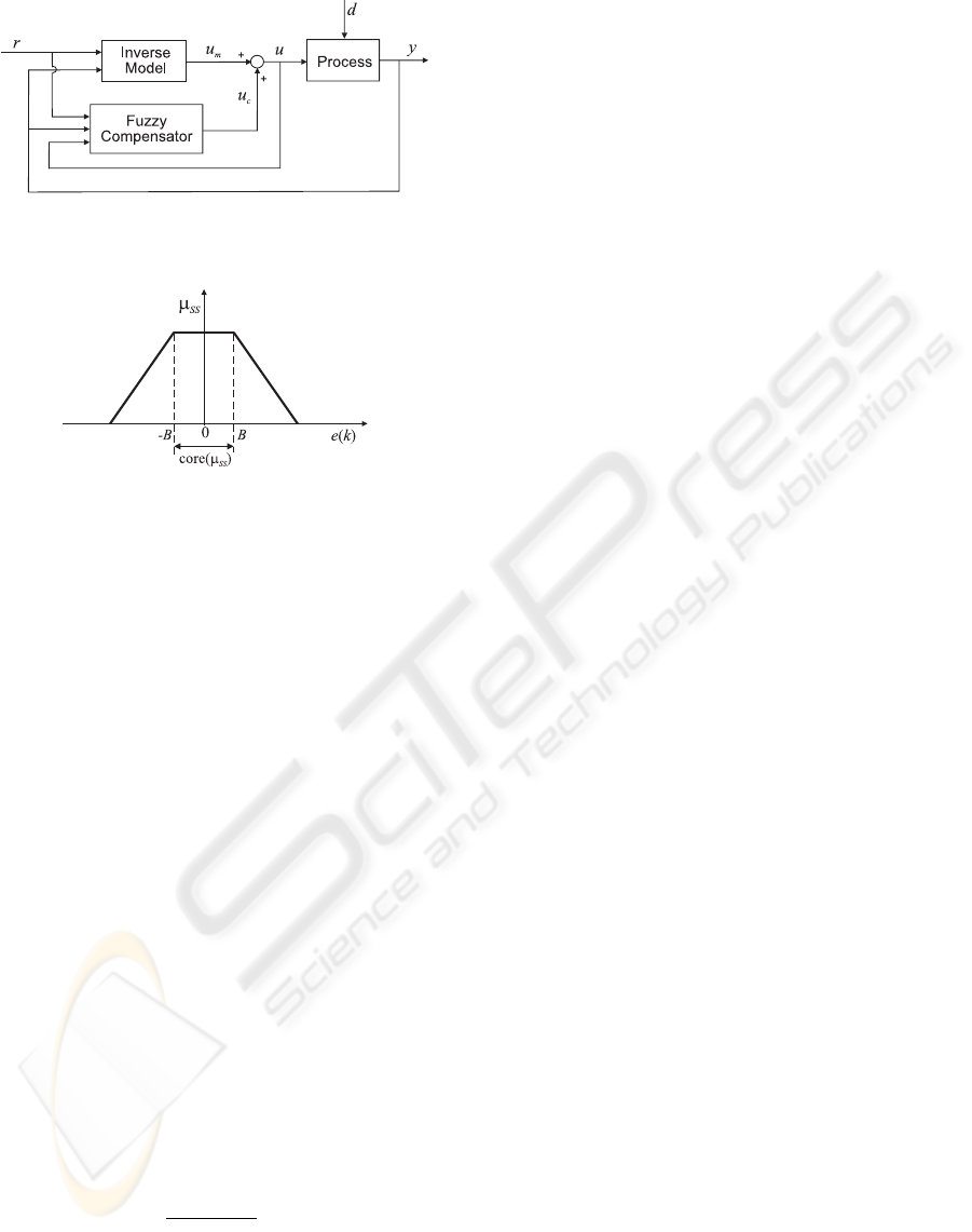
Figure 4: Fuzzy model-based compensation scheme.
Figure 5: Definition of the fuzzy boundary SS where fuzzy
compensation is active.
is defined as e(k)=r(k) − y(k), and the mem-
bership function µ
SS
(e(k)) is designed to allow for
steady-state error compensation whenever the support
of µ
SS
(e(k)) is not zero. The value of B that deter-
mines the width of the core(µ
SS
) should be an upper
limit of the absolute value of the possible steady-state
errors. Fuzzy compensation is fully active in the in-
terval [−B,B]. The support of µ
SS
(e(k)) should be
chosen such that it allows for a smooth transition from
enabled to disabled compensation. This smoothness
of µ
SS
induces smoothness on the fuzzy compensa-
tion action u
c
(k), and avoids abrupt changes in the
control action u(k).
The compensation action u
c
(k) at time k is given
by
u
c
(k)=µ
SS
(e(k))
k−1
i=0
u
c
(i)+Ke(k) f
−1
u
,
(22)
where µ
SS
(e(k)) is the error membership degree at
time k, K
c
is a constant parameter to be determined
and
f
u
=
∂f
∂u(k − 1)
x(k−1)
(23)
is the partial derivative of the function f in (20) with
respect to the control action u(k − 1), for the present
state of the system x(k − 1).
6 EXPERIMENTAL SETUP
The experimental setup can be divided in two subsys-
tems, the vision system and the robotic manipulator
system. The vision system acquires and process im-
ages at 50Hz, and sends image features, in pixels, to
the robotic manipulator system via a RS-232 serial
port, also at 50 Hz. The robotic manipulator system
controls the 2 dof planar robotic manipulator, Fig. 6
and Fig. 1 using the image data sent from the vision
system.
6.1 Vision System
The vision system performs image acquisition and
processing under software developed in Visual
C++
TM
and running in an Intel Pentium IV
TM
, at 1.7
GHz, using a Matrox Meteor
TM
frame-grabber. The
CCD video camera, Costar, is fixed in the robot end-
effector looking up and with its optical axis perpen-
dicular to the plane of the robotic manipulator. The
planar target is parallel to the plane of the robot, and
is above it. This configuration allows defining the Z
variable as pre-measured constant in the image Jaco-
bian (6) calculation, Z =1. The target consists of one
light emitting diode (LED), in order to ease the image
processing and consequently diminish its processing
time, because we are mainly concerned in control al-
gorithms.
Following the work in (Reis et al., 2000) the im-
age acquisition is performed at 50 Hz. It is well
known that the PAL video signal has a frame rate of
25 frames/second. However, the signal is interlaced,
i.e., odd lines and even lines of the image are codified
in two separate blocks, known as fields. These fields
are sampled immediately before each one is sent to
the video signal stream. This means that each field
is an image with half the vertical resolution, and the
application can work with a rate of 50 frames/second.
The two image fields were considered as separate im-
ages thus providing a visual sampling rate of 50 Hz.
When performing the centroid evaluation at 50 Hz,
an error on its vertical coordinate will arise, due to
the use of only half of the lines at each sample time.
Multiplying the vertical coordinate by two, we obtain
a simple approximation of this coordinate.
The implemented image processing routines ex-
tract the centroid of the led image. Heuristics to track
this centroid, can be applied very easily (Gonc¸alves
and Pinto, 2003b). These techniques allow us to cal-
culate the image features vector s, i.e., the two im-
age coordinates of the centroid. The image process-
ing routines and the sending commands via the RS-
232 requires less than 20ms to perform in our system.
The RS-232 serial port is set to transmit at 115200
bits/second. When a new image is acquired, the pre-
FUZZY MODEL BASED CONTROL APPLIED TO IMAGE-BASED VISUAL SERVOING
147
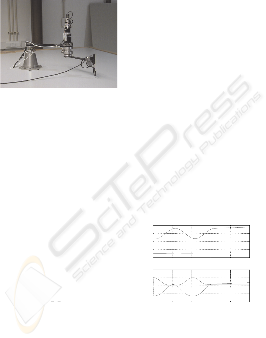
Figure 6: : Experimental Setup, Planar Robotic Manipula-
tor with eye-in-hand, camera looking up.
vious one was already processed and the image data
sent via RS-232 to the robotic manipulator system.
6.2 Robotic Manipulator System
The robot system consists of a 2 dof planar robotic
manipulator (Baptista et al., 2001) moving in a hor-
izontal plane, the power amplifiers and an Intel
Pentium
TM
200MHz, with a ServoToGo
TM
I/O card.
The planar robotic manipulator has two revolute joints
driven by Harmonic Drive Actuators - HDSH-14.
Each actuator has an electric d.c. motor, a harmonic
drive, an encoder and a tachogenerator. The power
amplifiers are configured to operate as current ampli-
fiers. In this functioning mode, the input control sig-
nal is a voltage in the range ±10V with current ratings
in the interval [−2; 2]V . The signals are processed
through a low cost ISA-bus I/O card from ServoToGo,
INC. The I/O board device drivers were developed at
the Mechanical Engineering Department from Insti-
tuto Superior T
´
ecnico. The referred PC is called in
our overall system as the Target PC. It receives the im-
age data from the vision system via RS-232, each 20
ms, and performs, during the 20 ms of the visual sam-
ple time, the visual servoing algorithms developed in
the Host-PC.
It is worth to be noted that the robot manipulator
joint limits are: q ∈ [−
π
2
;
π
2
].
6.3 Systems Integration
The control algorithms for the robotic manipulator
are developed in a third PC, called Host-PC. An exe-
cutable file containing the control algorithms is then
created for running in the Target-PC. The executable
file created, containing the control algorithm, is then
downloaded, via TCP/IP, to the Target-PC, where all
the control is performed. After a pre-defined time for
execution, all the results can be uploaded to the Host-
PC for analysis. During execution the vision system
sends to the Target PC the actual image features as a
visual feedback for the visual servoing control algo-
rithm, using the RS-232 serial port.
7 RESULTS
This section presents the simulation results obtained
for the robotic manipulator, presented in Section 6.
First, the identification of the inverse fuzzy model of
the robot is described. Then, the control results using
the fuzzy model based controller introduced in this
paper, i.e. the combination of inverse fuzzy control
and fuzzy compensation, are presented.
7.1 Inverse Fuzzy Modeling
In order to apply the controller described in this paper,
first an inverse fuzzy controller must be identified.
Recall that a model must be identified for each trajec-
tory. This trajectory is presented in Fig. 10. The pro-
file chosen for the image features velocity moves the
robot from the initial joints position q =[−1.5; 0.3]
to the final position q =[−1.51; 1.52], in one sec-
ond, starting and ending with zero velocity. An in-
verse fuzzy model (16) for this trajectory is identified
using the fuzzy modeling procedure described in Sec-
tion 4.1. The measurements data is obtained from a
simulation of the planar robotic manipulator eye-in-
hand system.
0 50 100 150 200 250
−2
−1
0
1
2
No samples [20 ms]
Joint Positions [rad]
Inverse Fuzzy Model Input Data
0 50 100 150 200 250
−0.1
−0.05
0
0.05
0.1
No samples [20 ms]
Image features velocity [m/s]
Figure 7: Input data for fuzzy identification. Top: joint po-
sitions, q. Bottom: image feature velocity, δs.
The set of identification data used to build the in-
verse fuzzy model contains 250 samples, with a sam-
ple time of 20ms. Figure 7 presents the input data,
which are the joint positions q
1
(k) and q
2
(k), and the
image features velocities δs
x
(k) and δs
y
(k), used for
identification.
ICINCO 2004 - INTELLIGENT CONTROL SYSTEMS AND OPTIMIZATION
148
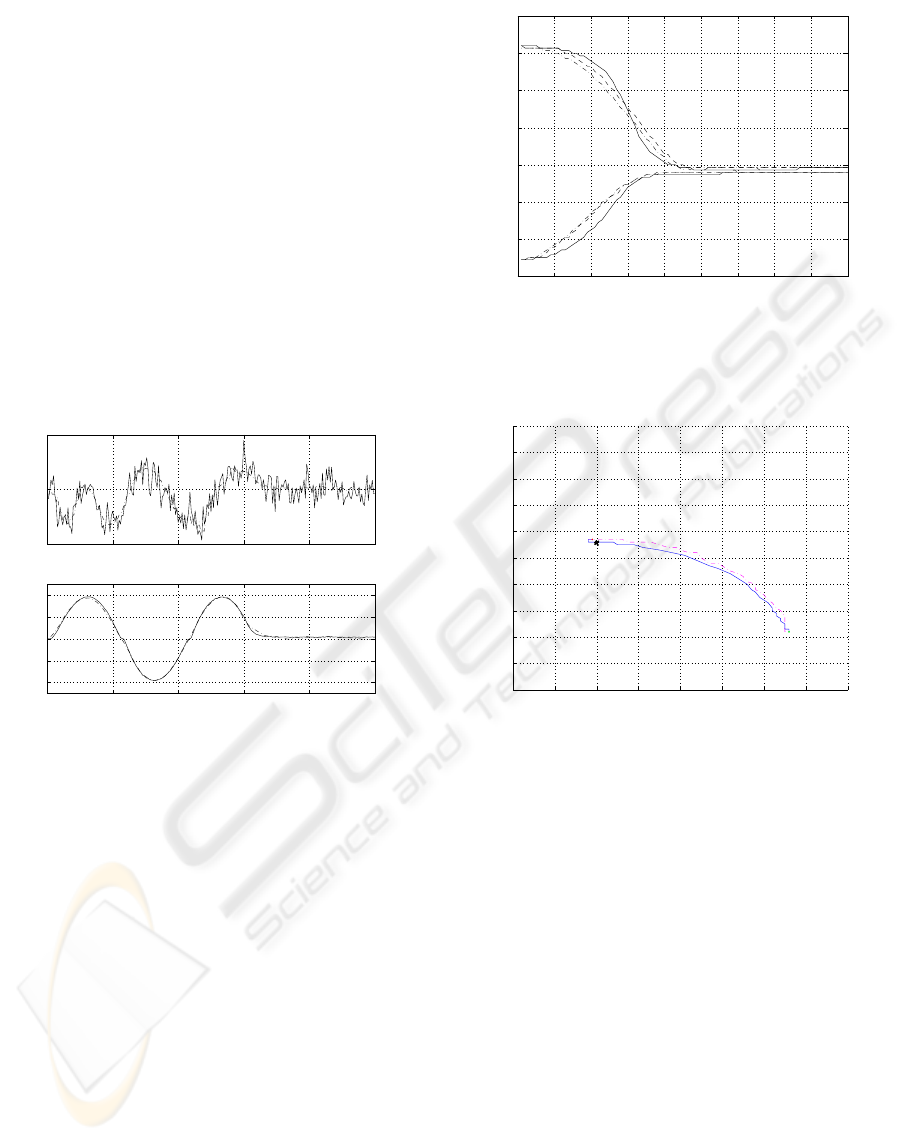
Note that to identify the inverse model, one cannot
simply feed the inputs as outputs and the outputs as
inputs. Since the inverse model (16) is a non-causal
model, the output of the inverse model must be shifted
one step, see (Sousa et al., 2003). The validation of
the inverse fuzzy model is shown in Fig. 8, where the
joint velocities δq are depicted. Note that two fuzzy
models are identified, one for each velocity. It is clear
that the model is quite good. Considering, e.g. the
performance criteria variance accounted for (VAF),
the models have the VAFs of 70.2% and 99.7%. When
a perfect match occur, this measure has the value of
100%. Then, the inverse model for the joint velocity
δq
2
is very accurate, but the inverse model for δq
1
is
not so good. This was expectable as the joint velocity
δq
1
varies much more than δq
2
. However, this model
will be sufficient to obtain an accurate controller, as is
shown in Section 7.2.
0 50 100 150 200 25
0
−0.05
0
0.05
No samples [20 ms]
Joint 1 Velocity [rad/s]
Inverse Fuzzy Model Validation
0 50 100 150 200 25
0
−2
−1
0
1
2
No samples [20 ms]
Joint 2 Velocity [rad/s]
Figure 8: Validation of the inverse fuzzy model (joint veloc-
ities δq). Solid – real output data, and dash-dotted – output
of the inverse fuzzy model.
In terms of parameters, four rules (clusters) re-
vealed to be sufficient for each output, and thus the
inverse fuzzy model has 8 rules, 4 for each output, δq
1
and δq
2
. The clusters are projected into the product-
space of the space variables and the fuzzy sets A
ij
are
determined.
7.2 Control results
This section presents the obtained control results, us-
ing the classical image-based visual servoing pre-
sented in Section 2, and the fuzzy model-based con-
trol scheme combining inverse model control pre-
sented in Section 4, and fuzzy compensation de-
scribed in Section 5. The implementation was devel-
oped in a simulation of the planar robotic manipula-
tor eye-in-hand system. This simulation was devel-
oped and validated in real experiments, using clas-
sic visual servoing techniques, by the authors. Re-
0 10 20 30 40 50 60 70 80 9
0
−0.06
−0.04
−0.02
0
0.02
0.04
0.06
0.08
No samples [20 ms]
Image Features Position [m]
Comparison of Image Features Position versus Trajectory
Figure 9: Image features trajectory, s. Solid – fuzzy visual
servo control; dashed – classical visual servo control, and
dash-dotted – desired trajectory.
−20 −10 0 10 20 30 40 50 6
0
−60
−50
−40
−30
−20
−10
0
10
20
30
40
Comparison of Image Features Trajectory
u [pixel]
v [pixel]
Figure 10: Image features trajectory s, in the image plane.
Solid – inverse fuzzy model control, and dash-dotted – clas-
sical visual servo control.
call that the chosen profile for the image features ve-
locity moves the robot from the initial joints position
q =[−1.5; 0.3] to the final position q =[−1.51; 1.52]
in one second, starting and ending with zero velocity.
The comparison of the image features trajectory for
both the classic and the fuzzy visual servoing con-
trollers is presented in Fig. 9. In this figure, it is shown
that the classical controller follows the trajectory with
a better accuracy than the fuzzy controller. However,
the fuzzy controller is slightly faster, and reaches the
vicinity of the target position before the classical con-
troller. The image features trajectory in the image
plane is presented in Fig. 10, which shows that both
controllers can achieve the goal position (the times,
×, sign in the image) with a very small error. This
figure shows also that the trajectory obtained with the
inverse fuzzy model controller is smoother. There-
fore, it is necessary to check the joint velocities in
order to check their smoothness. Thus the joint veloc-
FUZZY MODEL BASED CONTROL APPLIED TO IMAGE-BASED VISUAL SERVOING
149
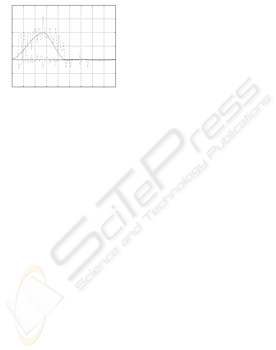
0 10 20 30 40 50 60 70 80 9
0
−2
−1
0
1
2
3
4
No samples [20 ms]
Joint Velocity [rad/s]
Comparison of Joint Velocities
Figure 11: Joint velocities, δq. Solid – fuzzy visual servo,
and dashed – classical visual servo.
ities are depicted in Fig. 11, where it is clear that the
classical controller presents undesirable and danger-
ous oscillations in the joint velocities. This fact is due
to the high proportional gain that the classical con-
troller must have to follow the trajectory, which de-
mands high velocity. This effect is easily removed by
slowing down the classical controller. But in this case,
the fuzzy controller clearly outperforms the classical
controller. The classical controller can only follow
the trajectory without oscillations in the joint veloc-
ities if the robot takes 1.5s to move from one point
to the other. In this case, the classical controller is
about 50% slower than the fuzzy model-based con-
troller proposed in this paper.
8 CONCLUSIONS
This paper introduces an eye-in-hand image-based vi-
sual servoing scheme based on fuzzy modeling and
control. The fuzzy modeling approach was applied
to obtain an inverse model of the mapping between
image features velocities and joints velocities. This
inverse model is added to a fuzzy compensator to be
directly used as controller of a robotic manipulator
performing visual servoing, for a given image features
velocity profile.
The obtained results showed that both the classi-
cal and the fuzzy controllers can follow the image
features velocity profile. However, the proportional
gain of the classic visual servoing must be very high.
This fact justifies the oscillations verified in the joint
velocities, which are completely undesirable in robot
control. For that reason, the inverse fuzzy control pro-
posed in this paper performs better.
As future work, the proposed fuzzy model based
control scheme will be implemented in the experi-
mental test-bed. Note that an off-line identification
of the inverse fuzzy model must first be performed.
The complete automation of this identification step is
also under study.
ACKNOWLEDGEMENT
This work is supported by the “Programa de Financia-
mento Plurianual de Unidades de I&D (POCTI) do Quadro
Comunit
´
ario de Apoio III”, by program FEDER, by the
FCT project POCTI/EME/39946/2001, and by the “Pro-
grama do FSE-UE, PRODEP III, acc¸
˜
ao 5.3, no
ˆ
ambito do
III Quadro Comunit
´
ario de apoio”.
REFERENCES
Babu
ˇ
ska, R. (1998). Fuzzy Modeling for Control. Kluwer
Academic Publishers, Boston.
Baptista, L., Sousa, J. M., and da Costa, J. S. (2001). Fuzzy
predictive algorithms applied to real-time force con-
trol. Control Engineering Practice, pages 411–423.
Espiau, B., Chaumette, F., and Rives, P. (1992). A new
approach to visual servoing in robotics. IEEE Trans-
actions on Robotics and Automation, 8(3):313–326.
Gonc¸alves, P. S. and Pinto, J. C. (2003a). Camera con-
figurations of a visual servoing setup, fora2dof
planar robot. In Proceedings of the 7th Interna-
tional IFAC Symposium on Robot Control, Wroclaw,
Poland., pages 181–187, Wroclaw, Poland.
Gonc¸alves, P. S. and Pinto, J. C. (2003b). An experi-
mental testbed for visual servo control of robotic ma-
nipulators. In Proceedings of the IEEE Conference
on Emerging Technologies and Factory Automation,
pages 377–382, Lisbon, Portugal.
Gustafson, D. E. and Kessel, W. C. (1979). Fuzzy clustering
with a fuzzy covariance matrix. In Proceedings IEEE
CDC, pages 761–766, San Diego, USA.
Hutchinson, S., Hager, G., and Corke, P. (1996). A tuto-
rial on visual servo control. IEEE Transactions on
Robotics and Automation, 12(5):651–670.
Reis, J., Ramalho, M., Pinto, J. C., and S
´
a da Costa, J.
(2000). Dynamical characterization of flexible robot
links using machine vision. In Proceedings of the 5th
Ibero American Symposium on Pattern Recognition,
pages 487–492, Lisbon, Portugal.
Sousa, J. M., Silva, C., and S
´
a da Costa, J. (2003). Fuzzy
active noise modeling and control. International Jour-
nal of Approximate Reasoning, 33:51–70.
Suh, I. and Kim, T. (1994). Fuzzy membership function
based neural networks with applications to the visual
servoing of robot manipulators. IEEE Transactions on
Fuzzy Systems, 2(3):203–220.
Tahri, O. and Chaumette, F. (2003). Application of moment
invariants to visual servoing. In Proceedings of the
IEEE Int. Conf. on Robotics and Automation, pages
4276–4281, Taipeh, Taiwan.
ICINCO 2004 - INTELLIGENT CONTROL SYSTEMS AND OPTIMIZATION
150
