
SOME FEASIBILITY ISSUES RELATED TO CONSTRAINED
GENERALIZED PREDICTIVE CONTROL
Sorin Olaru
*
and Didier Dumur
Supelec – Automatic Control Department, Plateau de Moulon, F 91 192 Gif sur Yvette cedex, France
Keywords: Generalized Predictive Control, Feasibility, Polyhedral Representation, Parametric Programming
Abstract This paper analyzes the feasibility of the generalized predictive control law under constraints on the input,
output or other auxiliary signals that depend linearly on the system variables. These constraints are
formulated as sets of linear equalities or inequalities; the control sequence is therefore elaborated based on a
quadratic optimization problem. The feasibility issues are related on one hand to the well posedness feature,
and on the other hand to the compatibility with the set-point constraints. The prediction of the feasibility is
of great interest from this point of view and necessary feasibility conditions are presented. Two possible
approaches are followed, one strictly related to the specific set-point and the second, more general,
examines the geo-metrical description of the optimization domain. The main practical advantage is that all
the results are based on off-line numerical procedures offering qualitative information prior to the effective
implementation.
1 INTRODUCTION
The computer aided design of control laws must
overcome important difficulties when some imposed
constraints must be satisfied. These constraints may
be forced by practical considerations as limitations
on the input control signal amplitude or rate. Other
constraints may arise from the qualities desired for
the control law, a classical example being the output
constraints (Maciejowski, 2002). Other hidden
constraints, from the end-user point of view, could
be forced for example with end-point stability
constraints.
All can be expressed as linear equality or
inequality constraints that have to be further
considered in the control design procedure
(Erhlinger, et al., 1996). This set describes in fact a
polyhedral domain for which a dual representation in
terms of generators is available (Wilde, 1993).
Analyzing the geometry and the evolutions of this
polyhedron due to the dynamic evolution of the
controlled system variables could highlight the
characterization of the control algorithm.
This paper considers the model predictive
control (MPC) in the presence of such operational
constraints that alienate the performance of the
control sequence provided by the unconstrained
optimum. The effects could be severe, as for
example unstable systems regulated by a constrained
controller cannot be stabilized for all initial
conditions. An exhaustive analysis of the system of
constraints may reveal useful properties such as the
expression of the “switching surfaces” for the linear
control laws and the corresponding affine
formulations (Bemporad, et al., 2002), (Seron, et al.,
2003). This paper deals with another important
aspect related to the constraints analysis, the
feasibility of the optimization problem to be solved
(Kouvaritakis, et al., 2000). This is a sensitive one as
long as, in the case of an infeasibility message
coming from the optimization solver, the entire
control law is invalidated and the control
performances are damaged in an irreversible way.
Consequently, an analysis of the infeasibility is
crucial for the validation of the predictive control
law (Olaru and Dumur, 2003), (Scokaert and Clarke,
1994b). This is equivalent with an off-line prediction
of infeasibility. It must be mentioned that even for
the analytical close form description the feasibility
domain represents an important problem.
The main contribution of this paper is to provide
results towards feasibility and to stress their
implications in the case of general types of set-
points. Theoretical aspects related to some classes of
necessary feasibility conditions are covered and an
algorithm is built in order to check these conditions,
based on off-line information. In practice, although
*)
The first author would like to acknowledge the support received
from the European Commission, Directorate General for Research.
70
Olaru S. and Dumur D. (2004).
SOME FEASIBILITY ISSUES RELATED TO CONSTRAINED GENERALIZED PREDICTIVE CONTROL.
In Proceedings of the First International Conference on Informatics in Control, Automation and Robotics, pages 70-77
DOI: 10.5220/0001135400700077
Copyright
c
SciTePress

it cannot be analytically proved that they are
sufficient, these conditions offer a good test for the
on-line feasibility. The advantage of this approach is
that it covers the CGPC feasibility directly linked
with the structure of the set-points to be followed.
The paper concludes with a numerical example
proving the usefulness of the specified procedures.
The paper is organized as follows: Section 2
describes the generalized predictive control
formulation. Section 3 examines the constrained
case and provides some basic results about
feasibility. Section 4 is dedicated to the geometrical
description of the constraints and the main results
towards necessary conditions to be satisfied for on-
line feasibility. Section 5 presents a simulation on a
second order non minimum phase system. Finally,
Section 6 gives some concluding remarks.
2 GENERALIZED PREDICTIVE
CONTROL
Generalized predictive control (GPC) is part of the
long-range predictive control (LRPC) or model
predictive control (MPC) family (Rossiter, 2003).
All these controllers are based on the fact that the
process evolution can be predicted over a horizon
taking into account the history of the control inputs,
plant outputs and the potential future control
sequence. The quantification of suitability for the
predicted response is measured by a cost function
that considers the fitness with respect to the desired
characteristics. GPC is characterized by two major
characteristics. It uses first a CARIMA plant model
)()()(
)()()()(
11
11
−−
−−
+
+−=
qtqC
dtuqBtyqA
∆ξ
(1)
where u, y are the system input and output
respectively,
)(t
ξ
represents a centered Gaussian
white noise, d the system time delay, A and B are
polynomials in
1−
q (the backward shift operator) of
degree
a
n and
b
n , and
11
1)(
−−
−= qq
∆
.
Then the cost function to be minimized is
quadratic in the tracking error and control effort over
a receding horizon
[]
[]
∑∑
==
−+++−+=
u
N
j
N
Nj
jtujtwjtyJ
1
2
2
)1()()(
ˆ
2
1
∆λ
(2)
where
)(
ˆ
jty +
is the output prediction,
21
, NN are
the minimum and maximum costing horizon,
u
N
the control horizon,
λ
a control weighting factor
and w the setpoint.
Based on the model mentioned earlier and
following the ideas of GPC (Clarke, et al., 1987) an
optimal j-step ahead predictor can be constructed
444344421
444444344444421
response forced
1
response free
11
)1()(
)1()()()()(
ˆ
−++
+−+=+
−
=
−−
jtuqG
tuqHtyqFjty
j
l
jj
∆
∆
(3)
where the
jjj
HGF ,, polynomials are solutions of
the Diophantine equations
)()()()(
1)()()()(
1111
1111
−−−−−
−−−−−
=+
=+
qJqBqHqqG
qFqqJqAq
jj
j
j
j
j
j
∆
(4)
The index (2) is rewritten for optimization purpose
0
T
T
T
5.0
)()(
J
J
uuu
uuuu
++=
=+−+−+=
kfkQk
kkwlkGwlkG
λ
(5)
with the vector form of (3)
)()(
ˆ
tt
pastpastuu
uihyifkGlkGy
∆
++=+=
with:
⎥
⎥
⎥
⎦
⎤
⎢
⎢
⎢
⎣
⎡
+
+
=
⎥
⎥
⎥
⎦
⎤
⎢
⎢
⎢
⎣
⎡
+
+
=
⎥
⎥
⎥
⎦
⎤
⎢
⎢
⎢
⎣
⎡
−
=
⎥
⎥
⎥
⎦
⎤
⎢
⎢
⎢
⎣
⎡
−
−
=
⎥
⎥
⎥
⎦
⎤
⎢
⎢
⎢
⎣
⎡
−+
=
)(
)(
;
)(
ˆ
)(
ˆ
ˆ
;
)(
)(
)(
)(
)1(
)(;
)1(
)(
2
1
2
1
Ntw
Ntw
Nty
Nty
nty
ty
t
ntu
tu
t
Ntu
tu
a
past
b
past
u
u
MMM
MM
wyy
uk
∆
∆
⎥
⎥
⎥
⎥
⎥
⎦
⎤
⎢
⎢
⎢
⎢
⎢
⎣
⎡
=
⎥
⎥
⎥
⎦
⎤
⎢
⎢
⎢
⎣
⎡
=
⎥
⎥
⎥
⎦
⎤
⎢
⎢
⎢
⎣
⎡
−
−
=
+−
−
−
1
1
1
22
2
11
22
11
22
11
0
)()1(
)()1(
;
)1()1(
)1()1(
u
NNN
N
NN
aNN
aNN
bNN
bNN
gg
g
gg
nFF
nFF
nHH
nHH
LL
MML
MMOM
L
L
MM
L
L
MM
L
G
ifih
In the unconstrained case, the optimum of J derived
through analytical minimization is given by the
relation
fQk
1−
−=
u
. By applying the first control
action
)1(
u
k
of this optimal sequence and restarting
the procedure, a control law with improved
performances under a “two degrees of freedom”
polynomial RST form is obtained (Boucher and
Dumur, 1998). Such a formulation takes advantage
of all the properties related to a closed loop control
law as at each sampling instant it uses the new
measured values of the plant output.
SOME FEASIBILITY ISSUES RELATED TO CONSTRAINED GENERALIZED PREDICTIVE CONTROL
71

3 CONSTRAINED GPC
All these properties have to be reanalyzed when
constraints are taken into consideration (Camacho,
1993). The design procedures most often have to
consider specific types of constraints originated by
amplitude limits in the control signal, slew rate
limits of the actuator, limits on the output signal or
equality constraints at the end of the prediction
horizon for stability purposes.
3.1 Constraints formulation
Generally the formal mathematical description is
⎪
⎪
⎩
⎪
⎪
⎨
⎧
=+=++
≤≤≤+≤−
−≤≤≤+≤−
≤−+−+≤−
mkNtwkNty
NkNyktyy
Nkuktuu
uktuktuu
u
...1),()(
ˆ
,)(
ˆ
10,)(
)1()(
22
21maxmin
maxmin
maxmin
∆∆
(6)
These constraints on the control action and outputs
can be restated in a form depending only on control
updates. Further, this description could be translated
in a matrix form like in (Ehrlinger, et al., 1996)
⎪
⎪
⎪
⎩
⎪
⎪
⎪
⎨
⎧
+=+
≤+≤−
−−=−−−=
≤≤−
≤≤−
)()1,(
)1,()1,(
)1(),1(
,)1,()1,(
)1,()1,(
2
maxmin
maxmin
maxmin
Ntwm
yNyN
tuuutuuu
uNuN
uNuN
cuc
u
uuu
uuu
MlkG
MlkGM
MkLM
MkIM
∆∆
(7)
where
1
12
+−= NNN , ),( rqM is a matrix of
dimension
r
qx whose entries are one on the first
column and zero for the others,
L is a
uu
NN x
lower triangular matrix whose entries are one.
c
G
and
c
l
describe the dynamics and the free response
of the constrained system, both found as in (3), (5).
3.2 Feasibility
When minimizing the index J in (2) with respect to
the constraints, the methods presented in the relaxed
case cannot be applied since they do not provide a
solution when the global optimum violates the
constraints. In this case, practical GPC
implementation is dealing with nonlinearities in the
control law due to the entrance in the frontier
hyperspace of the polyhedral domain defined by the
set of constraints. These nonlinearities affect the
controller expression that is usually found by solving
on-line the quadratic program and applying then the
receding horizon principle. However, the control law
is affected irreversibly when on-line optimization
returns infeasibility messages as in this case no
pertinent control action can be applied.
Recalling the definition of the two types of
infeasibility (Olaru and Dumur, 2003), type I is easy
to analyze by a simple inspection of the optimization
domain. It is not the same for the type II infeasibility
as long as it depends on the set-point, which may
conflict with the system dynamics and the other
inequality constraints. Notice that there always
exists a set-point which causes the infeasibility of
the optimization for a system with a given set of
constraints.
3.3 Necessary conditions
The following result concerns the degrees of
freedom and the dynamics of the predicted output.
However, it does not give any insight for the
constrained domain point of view. To do that, a
geometrical approach must be examined, which will
be considered in Section 4. The optimization
problem to be solved at instant t will be noted here
))(,,,,( mNwmNNtP
u
+
. The argument for the
solution to this problem will be noted
))(,,,,( mNwmNNtK
u
+
.
The following proposition introduces a necessary
condition for feasibility of a GPC law.
Proposition 1: If a GPC law is feasible at each
instant
0>t , then the existence of all the following
sequences is assured
0)),(,,,,0( ≥∀++
+
+
kkmNwmkNkNK
u
(8)
Proof: GPC feasibility is equivalent with the
feasibility of
))(,,,,( mNwmNNtP
u
+ for any
t
and as result with the existence of the optimal
solution
))(,,,,( mNwmNNtK
u
+ .
For
0
=
t , ))(,,,,0( mNwmNNP
u
+ is feasible
and thus
))(,,,,0( mNwmNNK
u
+ exists which is
(8) for
0
=
k . Assume the existence of the first 1
−
k
))(,,,,0( imNwmiNiNK
u
+
+
+
+
, 10
−
= ki L ,
solutions. Based on the optimization problem until
time
k , the following sequence can be built
{
}
)1))((,,,,1(,
),1))((,,,,0(
mNwmNNkK
mNwmNNK
u
u
+−
+=ℵ
K
K
which is the sequence of the first
k GPC control
actions. On the other hand at instant
k , from the
hypothesis the CGPC law defines a feasible opti-
mization problem
))(,,,,( mNwmNNkP
u
+ with
solution
))(,,,,( mNwmNNkK
u
+ , adding it to the
existing
ℵ
, a kN
u
+
control sequence is obtained
{
}
))(,,,,(, mNwmNNkK
u
+ℵ=ℵ (9)
Each element of this vector satisfies the operational
constraints of
))(,,,,0( mkNwmkNkNP
u
+++
+
as
ICINCO 2004 - SIGNAL PROCESSING, SYSTEMS MODELING AND CONTROL
72
long as its set of constraints is included in the union
of all subsets upon which the elements of
ℵ
were
constructed. Now, as the final part of the sequence
ℵ
, ))(,,,,( mNwmNNkK
u
+ satisfies the end-point
constraints for
))(,,,,( mNwmNNkP
u
+ being the
same as for
))(,,,,0( mkNwmkNkNP
u
+
+
++ .
ℵ
is thus a feasible solution to this problem and
there exists
))(,,,,0( kmNwmkNkNK
u
+
+++ .
The result is completely proved by induction. ■
To illustrate how the result of Prop. 1 can be
exploited, consider a simple second order system
)()()25.01(
21
tutyqq =+−
−−
(10)
An unconstrained GPC law with horizons
1
1
=
N ,
4
2
=N , 2=
u
N controls without problems the
system for a pulse train set-point of magnitudes 0.3
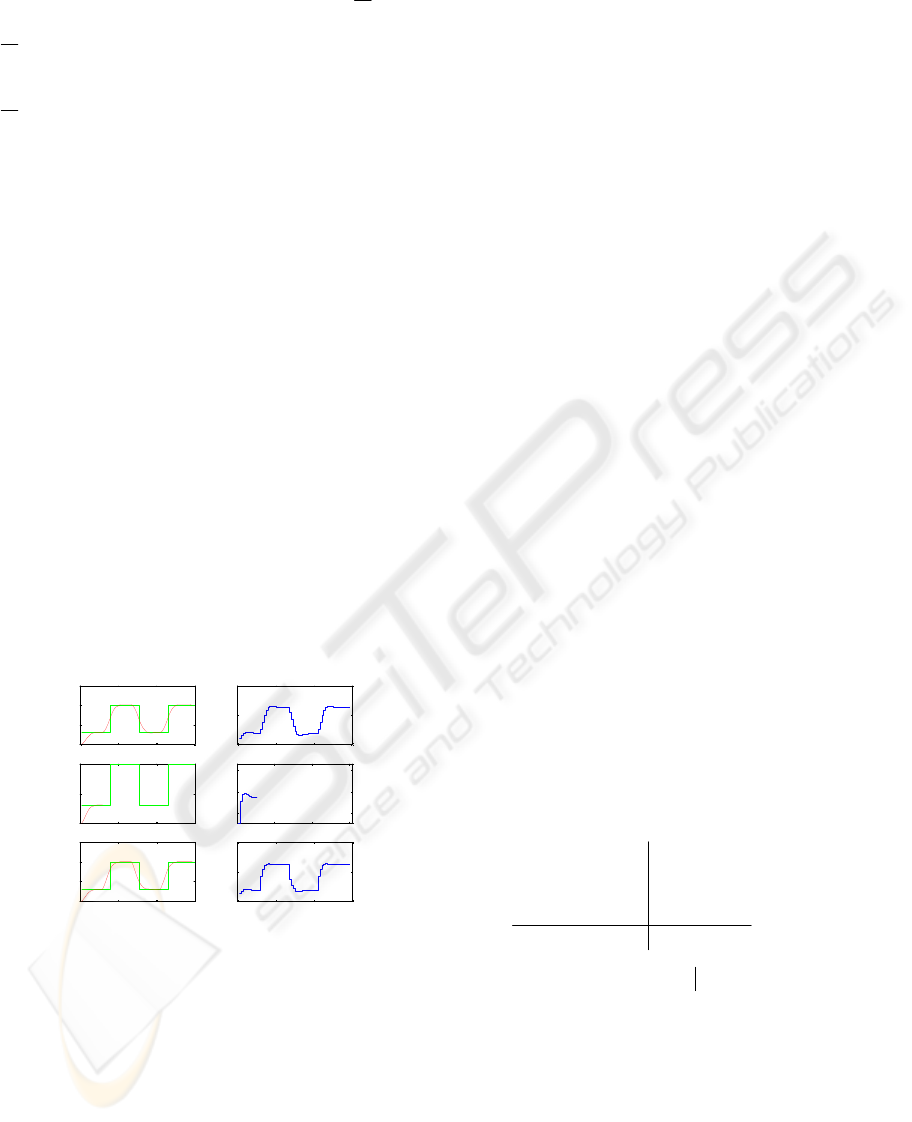
and 1 (Figures 1a, b). Similar performances are
available even if constraints on the input update
1.01.0 ≤≤− u
∆
are introduced. Difficulties arise
when endpoint constraints are added to the previous
ones (
1=m in the case of Figures 1c, d). The
second ascending front of the set-point requires an
important control effort to satisfy the endpoint
constraints and the control law in this constrained
case becomes infeasible. The infeasibility only
appears at the 12
th
iteration while from the necessary
condition it was obvious that as long as
))13(,,12,12,0( +++ NwmNNP
u
is infeasible, the
CGPC law is infeasible. Figures 1e, f shows that the
control law with only endpoint constraint is feasible.
0 20 40 60
0
0.5
1
1.5
e
0 20 40 60
0
0.2
0.4
f
0 20 40 60
0
0.5
1
1.5
a
0 20 40 60
0
0.2
0.4
b
0 20 40 60
0
0.5
1
c
20 40 60
0.06
0.08
0.1
d
y(t),w(t)
u(t)
Figure 1: a, b) Output, setpoint and input for GPC
c, d) output, setpoint and input for CGPC
e, f) output, setpoint and input for CGPC with endpoint
constraints only.
Generally, if for a set of GPC parameters there exists
a
k for which ))(,,,,0( mkNwmkNkNP
u
+
+
++
is infeasible, then there exists a
t
such that
))(,,,,( mNwmNNtP
u
+ is infeasible. In practice,
all
),,( mNN
u
combinations with this property must
be avoided. Thought these are useful principles, a
finite time procedure checking the necessary
conditions is not achievable in the general case.
However, the necessary condition can be checked
for some specific k values, which in the case of
regular set-points might cover all the possible cases
(see (Olaru and Dumur 2003) for a step set-point
example).
Furthermore, Prop. 1 considers necessary, but
not sufficient, feasibility conditions. With the same
previous system (10) with endpoint constraints, if
the set-point is a pulse train of magnitudes 0.35 and
35.0
−
, all the optimization problems (8) are feasible
but the GPC law is infeasible.
4 GEOMETRICAL ANALYSIS
More complex results towards sufficient feasibility
conditions based on invariant sets exist, which are
too conservative. Consequently, an alternative
approach in order to achieve some tractable
necessary conditions considers a dual representation
of the polyhedral domain coming from the
constraints.
4.1 Constrained domain evolution
Trying to describe the feasibility domain for a
system under all types of constraints, a compact
form is deduced from (7)
0Γ
Γ
Γ
θ
F
F
Γ
F
>
⎥
⎦
⎤
⎢
⎣
⎡
≤
⎥
⎦
⎤
⎢
⎣
⎡
−
;)(
min
max
~
43421
321
t
(11)
with
[]
T
max
max
max
max
max
min
min
min
min
min
)()()()()()(
0
00
000
0000
)1,(
)1,(
)1,(
)1,(
)1,(
)1,(
)1,(
)1,(
tttttt
m,n
,nN
m
yN
uN
uN
m
yN
uN
uN
cupastpast
wccc
bu
N
u
u
u
u
u
wwkuyθ
)M(Gih∆if
Gih∆if
L)M(
I
F
M
M
M
M
Γ
M
M
M
M
Γ
=
⎥
⎥
⎥
⎥
⎦
⎤
⎢
⎢
⎢
⎢
⎣
⎡
−
=
⎥
⎥
⎥
⎥
⎦
⎤
⎢
⎢
⎢
⎢
⎣
⎡
=
⎥
⎥
⎥
⎥
⎦
⎤
⎢
⎢
⎢
⎢
⎣
⎡
=
ε
∆
ε
∆
where the epsilon machine will represent the bounds
for equality constraints,
w
n is the required number
of past known values that are necessary to properly
evaluate the future setpoint evolution.
A possible way of modeling (11) considers the
dual representation of the inequalities in (7)
{
}
{}
spacePlinyycone
xxhullconvP
r
v
.,,
,,.
1
1
++
+=
K
K
(12)
SOME FEASIBILITY ISSUES RELATED TO CONSTRAINED GENERALIZED PREDICTIVE CONTROL
73

where conv.hullX denotes the set of all convex
combinations of points in X, coneY denotes
nonnegative combinations of unidirectional rays and
lin.spaceP represents a linear combination of bi-
directional rays. It can be rewritten as
ii
v
i
ii
l
i
ii
r
i
ii
v
i
ii
zyxP
µγλλ
µγλ
∀≥=≤≤
++=
∑
∑∑∑
=
===
,0,1,10
1
111
(13)
The complete procedure for finding the dual
representation evaluates the system of constraints
through Chernikova algorithm (Le Verge, 1992)
implemented in libraries like POLYLIB.
Usually the polyhedral domain related with
practical CGPC laws are in fact polytopes. These
domains in a compact form can be analysed by their
evolution, providing the dynamics of the constrained
variables vector. This is the purpose of the next part.
Let us before examine the explicit linear
controller structure. It comes from (5)
(
)
()
)(2
2
*
T
T
T
T
T
T
t
J
uuu
uuu
θEGkkIGGk
wlGkkIGGk
H
+
⎟
⎟
⎟
⎠
⎞
⎜
⎜
⎜
⎝
⎛
+=
=−++=
43421
λ
λ
(14)
where
E is a matrix which allows the description of
the vector
)(* tEθwl =− when
⎥
⎥
⎥
⎥
⎥
⎥
⎦
⎤
⎢
⎢
⎢
⎢
⎢
⎢
⎣
⎡
⎥
⎥
⎥
⎥
⎦
⎤
⎢
⎢
⎢
⎢
⎣
⎡
=
==
⎥
⎥
⎥
⎥
⎦
⎤
⎢
⎢
⎢
⎢
⎣
⎡
+
+
+
+
=+
)(
)(
)(
)(
)(
000
0000
000
00)()()(
)(
)1(
)1(
)1(
)1(
)1(
43
1
4
321
**
t
t
t
t
t
t
t
t
t
t
t
c
u
past
past
dev
c
past
past
w
w
k
u
y
MM
M
DI
GDihDifD
θΦ
w
w
u
y
θ
(15)
One can find the description for the vector
u
k
by
minimizing this index J under the constraints
)1(
*
−−≤ t
u
θKΦbkA (16)
where
K is a matrix allowing the description of the
affine part of the inequalities as a linear dependence
on the context parameters
)(
*
tθ . The close form of
the optimal control sequence for the CGPC is
()
=−−+
−−=
−−−
−−−−−
)1()(
)1())((*
*1
T
0
1
0
T
0
1
*11
0
1
T
0
1
0
T
0
1
t
t
u
θKΦbAHAAH
θGEΦHHAAHAAHk
bAHAAH
θKΦAHAAH
GEΦHHAAHAAH
1
T
0
1
0
T
0
1
*1
T
0
1
0
T
0
1
*11
0
1
T
0
1
0
T
0
1
)(
)1()(
)(
−−−
−−−
−−−−−
+
+−
⎥
⎦
⎤
−
⎢
⎣
⎡
⎟
⎠
⎞
⎜
⎝
⎛
−=
t
with
0
A
the matrix constructed by the subset of
lines in
A for whom the inequality constraints are
saturated.
As a conclusion, the elaborated control law is
affine in the parameter vector
)1( −tθ . However, the
difficulties arise from the fact that the matrix
))1((
00
−= tθAA is not allowing an explicit
dependence on the vector of parameters.
Remark: A parameterized polyhedron like the
one in (16)
{
}
)1(
*
−−≤= tP
uu
θKΦbkAk
has a dual representation where only the vertices are
affected by the parameters
⎪
⎪
⎭
⎪
⎪
⎬
⎫
⎪
⎪
⎩
⎪
⎪
⎨
⎧
∀≥=≥
++=
=
∑
∑∑∑
=
===
ii
v
i
ii
l
i
ii
r
i
ii
v
i
iiuu
zyx
P
µγλλ
µγλ
,0,1,0
)(
1
111
*
θkk
4.2 Necessary conditions by means of
extremal point feasibility
Considering the polyhedral domain as described
earlier, with the dual representation by the vertices,
it can be interesting to look at the evolution of these
vertices at each sampling time.
Proposition 2: The optimal control sequence
corresponding to all extremal combinations of
context parameters must lead to points inside the
projection of the initial polyhedral domain for a
feasible CGPC law.
Proof sketch: As explained earlier, the constraints
on the CGPC law define a polyhedral domain, given
in the case of a polytope by
⎪
⎭
⎪
⎬
⎫
⎪
⎩
⎪
⎨
⎧
=≥==
∑∑
==
v
i
ii
v
i
i
uiuu
kD
11
1,0;*)(
λλλ
θkk
(17)
By considering the involved system variables as
parameters, this parameterized polyhedron can be
extended to a fixed one of higher dimension. Fur-
ther, a corresponding representation as a generators
combination may be found. In the case of a
polytope, this will be
ICINCO 2004 - SIGNAL PROCESSING, SYSTEMS MODELING AND CONTROL
74
⎪
⎭
⎪
⎬
⎫
⎪
⎩
⎪
⎨
⎧
=≥==
∑∑
==
v
i
ii
v
i
ii
P
11
1,0;
λλλ
θθθ
(18)
The existence of these vertices does not guaranty the
fact that the CGPC law will have the opportunity to
reach each of them. Multiple vertices may
correspond to the same context parameters. Thus, a
useful manipulation may be the orthogonal
projection of this domain on the subspace of the
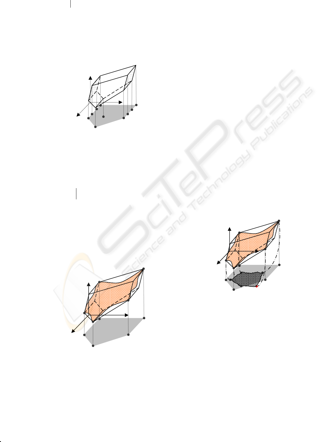
context parameters (as in Figure 2).
Figure 2: The polyhedral domain and its projection on the
context parameters subspace.
This operation can be done explicitly by
multiplying each vertex
i
θ
by a matrix
[
]
j
e where j
are the indices of the context parameters in the
vector
θ . The resulting set is
*
P
, the convex
combination of the points
[]
{
}
ij
eP
θ
==
***
θθ (19)
Once the projection available, a redundancy check
must be operated in order to obtain the minimal set
of generators.
The resulting domain
*
P
can provide by its
vertices the extremal points for the context parame-
ters that can further be used for figuring the whole
domain. Solving the parameterized quadratic
problem related to CGPC, one can retrieve a hyper
surface inside the original polyhedral domain
D
.
Figure 3: The optimal solution of CGPC for each possible
context parameters combination.
The elaboration of this shape enables to solve all the
analysis problems as it defines the whole behavior of
the CGPC law. However, this is not a trivial task
although systematic results exist at least for the
MPC with state space models. The investigated case
is slightly different as long as it incorporates also a
model of the reference, even if the optimization
problem is still a part of the quadratic multi-
parametric programs.
As far as the evolution of the context parameters
domain is concerned, the image of the points on the
CGPC shape must be found by the linear
transformation (15). If this domain is denoted as
*
+
P , the necessary and sufficient conditions for
feasibility are resumed by the relation
*
*
+
⊃ PP (20)
Due to limitations in the knowledge on the topology
of the CGPC shape, this will resume on necessary
conditions based on the extremal points. These
necessary conditions may be expressed as in Figure
4 by a set of inequalities
*
)1(*
+
∈+ Ptθ (21)
which resumes the proposition. ■
In practice this condition seems to be quite
general and covers with sufficiency all the special
cases verified by the authors. An analytical proof of
the fact that the extremal points of the CGPC shape
corresponding with the extended polyhedron vertices
will have as image the vertices of the domain
*
+
P
can not yet be obtained.
Figure 4: The evolution of the extremal points of context
parameters domain.
For a complete analysis of the CGPC law, all the
points inside the polyhedral domain
*
+
P have to be
checked in order to confirm the feasibility. This is
not an obvious task as long as the optimal control
sequence is affine in the context parameters, and the
affine part even if linear in the parameter vector is
changing the linear dependence in concordance with
the active set of constraints. It is clear that the
number of active constraints is maximal for the
θ
1
k
u
θ
1
k
u
θ
1
θ
n
θ
n
θ
n
k
u
SOME FEASIBILITY ISSUES RELATED TO CONSTRAINED GENERALIZED PREDICTIVE CONTROL
75
vertices and is subsequently decreasing for the
points on the frontier where subsets of these sets of
constraints are active.
Following the same line as the proof, an
algorithm based on tools of polyhedral computations
and quadratic optimization can be designed in order
to validate these necessary conditions. Such an
algorithm can be resumed by the following steps.
Algorithm 1
1. Compute the vertices of the polyhedral set by
dual representation of the constraints
2.
Project the polytope on the parameters subspace
3.
Remove the redundant points
4.
Compute the close form of the control law in all
the vertices of the constrained domain.
(Compulsatory as it is not always equal with the
value in the original polyhedron)
5.
For each such law, construct the evolution
matrix and compute the corresponding next step
parameters
)1( +tθ
6.
Check if for each such point
)1(
+
tθ
, its
projection is inside the projected polyhedron
found at step 2. If it is not the case, that means
that there exists at least one point in the
constrained domain which, if reached, will lead
to infeasibility. The necessary conditions are
thus not accomplished.
5 EXAMPLE
A simple constrained generalized predictive control
is examined in order to illustrate the analysis tech-
nique procedure proposed in the previous section.
Consider in the following a second order linear
system as the one reported in (Olaru and Dumur,
2003), with non-minimum phase characteristics
)()75.025.025.0(
)()25.01(
21
21
tuqq
tyqq
−−
−−
+−−
=+−
(22)
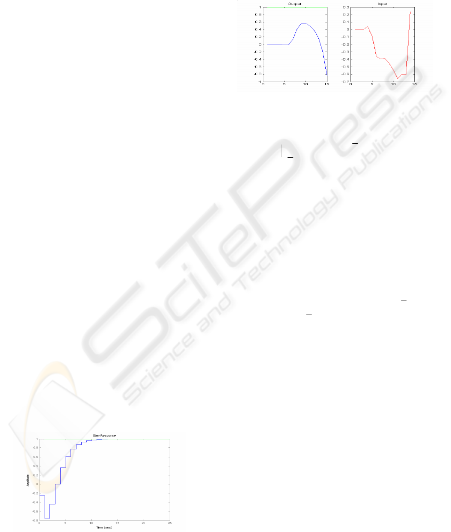
Figure 5: Open loop step response.
The step response of this system is given in Figure 5.
For CGPC law with
1
1
=
N , 4
2
=N , 2=
u
N , the
system proves to have an infeasible behavior for step
setpoints and constraints on the output of magnitude
11
≤
≤
−
y , based on snow-ball attitude (Scokaert
and Clarke, 1994a) (Figure 6).
Figure 6: CGPC closed loop behavior.
Proceeding as explained in Algorithm 1, the
constrained domain can be described as
{
}
yyD
uu
1lkG1k ≤+≤= (23)
where
l is like in (3) and
⎥
⎥
⎥
⎥
⎦
⎤
⎢
⎢
⎢
⎢
⎣
⎡
−
−−
−−
−
=
40.00
80.040.0
25.075.0
025.0
G
(24)
The elaboration of the extended polyhedron requires
the definition of
{
}
0ΓΓΓθFΓ ≥
≤
≤
−
=
maxminmaxmin
,)(tP (25)
with:
TT
T
max
TT
T
min
; 11Γ11Γ ==== yy
[]
T
)()()()(
4.004.22.18.04.36.3
8.04.028.07.032.3
25.075.05.125.05.025.275.2
025.075.025.025.025.12
tttt
upastpast
kuyθ
F
∆
=
⎥
⎥
⎥
⎥
⎦
⎤
⎢
⎢
⎢
⎢
⎣
⎡
−−−−
−−−
−−−
−−−
=
As the context parameters include the past outputs,
three implicit constraints have been added as an
upper part of F in order to avoid the analysis of non-
reachable regions. The result is a square matrix of
constraints describing a polytope with a dual
representation containing 128 vertices
θ
1
= [ 148 -148 -148 -59 -467 -158 -315 ]/148
θ
2
= [-148 148 -148 -459 689 -138 241 ]/148
θ
3
= [ 148 148 148 -309 15 354 -97 ]/148
…
θ
128
= [-148 -148 148 -357 207 90 23 ]/148
Figure 7: Convex hull for D computed by POLYLIB.
ICINCO 2004 - SIGNAL PROCESSING, SYSTEMS MODELING AND CONTROL
76

Now the projection on the subspace of the first five
variables leads to a domain
*
P
that can be reduced
by removing redundant pairs to the convex hull of
64 vertices like in Figure 8.
θ
1
= [-148 -148 148 335 -193 ]/148
θ
2
= [ 148 148 -148 677 -303 ]/148
θ
3
=[ 148 -148 -148 793 -767 ]/148
…
θ
64
= [-148 148 148 -793 767 ]/148
Figure 8: Convex hull for P
*
computed by POLYLIB.
Now the corresponding quadratic problems have to
be solved in order to find the optimal control law in
each such extreme context.
The next step aims at
computing the image of the resulting extended
vectors
64..1
θ
by the linear transformation
⎥
⎥
⎥
⎦
⎤
⎢
⎢
⎢
⎣
⎡
⎥
⎥
⎥
⎥
⎥
⎥
⎦
⎤
⎢
⎢
⎢
⎢
⎢
⎢
⎣
⎡
−−−
=
=
⎥
⎦
⎤
⎢
⎣
⎡
+
+
=+
)(
)(
)(
0001000
0010000
0000010
0000001
025.075.025.025.025.12
)1(
)1(
)1(*
t
t
t
t
t
t
u
past
past
past
past
k
u
y
u
y
θ
∆
∆
Checking their membership inside D ends the
algorithm. In the studied case, there are 32 vertices
which are positioned outside the feasible context
polyhedron
*
P
. This means that there are at least 32
combinations of past inputs and outputs for which
there is no feasible control sequence able to retain
the system inside the constraints
11 ≤≤− y
Thus as the necessary conditions are not fulfilled,
the overall CGPC law is infeasible.
6 CONCLUSION
This paper presented some possible approaches for
the off-line analysis of the feasibility in the case of a
constrained generalized predictive control strategy.
The advantages of these kinds of analysis consist in
the set-point dependent procedure that may prove to
be useful in the decisions of tuning predictive
control law parameters.
However, a gap between the necessary and
sufficient conditions for off-line feasibility of CGPC
exists as long as the dependence of affine linear
control law corresponding to the saturated
constraints as functions of the context parameters
can not be explicitly computed.
REFERENCES
Bemporad, A., Morari, M., Dua, V. and Pistikopoulos, E.,
2002. The explicit linear quadratic regulator for
constrained systems, Automatica, Volume No 38, pp.3-
20.
Camacho, E.F., 1993. Constrained Generalized Predictive
Control, IEEE Transactions on Automatic Control,
Volume No 38-2, pp.327-331.
Clarke, D.W., Mohtadi C., and Tuffs, P.S., 1987.
Generalised Predictive Control: Part I: The Basic
Algorithm, Part II: Extensions and Interpretation,
Automatica, Volume No 23-2, pp.137-160.
Dumur D. and Boucher, P., 1998. A Review Introduction
to Linear GPC and Applications, Journal A, Volume
No 39-4, pp.21-35.
Ehrlinger, A., Boucher, P. and Dumur, D., 1996. Unified
Approach of Equality and Inequality Constraints in
G.P.C.. 5
th
IEEE Conference on Control Applications,
pp.893-899, Dearborn, September.
Kouvaritakis, B., Cannon, M. and Rossiter, J.A., 2000.
Stability, feasibility, optimality and the degrees of
freedom in constrained predictive control, in
Nonlinear Model Predictive Control, F. Allgower and
A. Zheng (eds.), Progress in Systems and Control
Theory Series, Volume No 26, pp.403-417, Birkhauser
Verlag, Bâle.
Le Verge, H., 1992. A note on Chernikova's Algorithm,
Technical Report 635, IRISA-Rennes, France.
Maciejowski, J., 2002. Predictive Control with
Constraints, Prentice Hall.
Olaru, S., and Dumur, D., 2003. Feasibility analysis of
constrained predictive control, 14
th
Conference on
Control Systems and Computer Sciences, pp.164-169,
Bucharest, July 2003.
Rossiter, J.A., 2003. Model based predictive control – a
practical approach, CRC Press.
Scokaert, P. and Clarke, D.W., 1994a. Stability and
feasibility in constrained predictive control, In:
Advances in model-based predictive control, pp.217-
230. Oxford University Press.
Scokaert, P. and Clarke, D.W., 1994b. Stabilising
properties of constrained predictive control, IEE
Proceedings Control Theory Applications, Volume
No 141-5, pp.295-304, September.
Seron, M.M., Goodwin, G.C. and De Dona, J.A., 2003.
Characterisation of Receding Horizon Control for
Constrained Linear Systems, Asian Journal of
Control, Volume No 5-2, pp. 271-286.
Wilde, D.K., 1993. A library for doing polyhedral
operations, Technical report 785, IRISA-Rennes,
France.
SOME FEASIBILITY ISSUES RELATED TO CONSTRAINED GENERALIZED PREDICTIVE CONTROL
77
