
MOBILE ROBOT LOCALIZATION BY CONSTRAINT
PROPAGATION ON INTERVALS
Mélanie Delafosse, Arnaud Clérentin, Laurent Delahoche, Eric Brassart
IUT, département Informatique
Avenue des Facultés le Bailly, 80025 AMIENS cedex – FRANCE
Keywords: Mobile robot localization, interval analysis, constraint propagation, data fusion
Abstract: This paper proposes to use constraint propagation on intervals to solve the mobile robot localization
problem. The mobile robot is equipped with an exteroceptive sensor and dead-reckoning. These two sensors
give imprecise data that are modelled by intervals. Our localization strategy is based on multi target tracking.
To this aim, the data given by our two sensors are fused by constraint propagation. So, at the end of the
localization process, we get a 3-D subpaving which is supposed to contain the robot’s position in a
guaranteed way. The localization imprecision is naturally managed by our method.
1 INTRODUCTION
Localization is a preponderant problem in mobile
robotics. Mobile robots have to be able to locate
themselves in their environment in order to
accomplish their mission. But the knowledge of the
robot’s position is not sufficient. An estimation of
the uncertainty and the imprecision of this position
should be determined and taken into account in
order to act in a robust way. In other words, the
decisions about the robot’s behaviour should be
made considering an uncertainty and an imprecision
about the robot localization. The aim is to increase
the reliability in operation, that is to say to assure the
success of the mobile robot mission.
The two notions of uncertainty and imprecision
are distinct ones and they must be clearly define.
The imprecision results from unavoidable
imperfections of the sensors and of the environment
map, i.e. the imprecision represents the error
associated to the measurement of a value. For
example, “the weight of the object is between 1 and
1.5 kg” is an imprecise proposition. On the other
hand, the uncertainty represents the belief or the
doubt we have on the existence or on the validity of
a data. This uncertainty comes from the reliability of
the observation made by the system: this observation
can be uncertain or erroneous. In other words, the
uncertainty denotes the truth of a proposition. For
example, “John is perhaps in the kitchen” is an
uncertain proposition.
The management of the uncertainty has been
already done in previous work (Clérentin,
2001)(Clérentin, 2002). The key tool used in this
purpose is the Transferable Belief Model (Smets,
1998), a non probabilistic variant of the Dempster-
Shafer theory. Indeed, this theory enables to easily
treat uncertainty since it permits to attribute mass
not only on single hypothesis, but also on union of
hypothesis. We can thus express ignorance. So it has
enabled us to manage and propagate an uncertainty
from low level data (sensor data) in order to get a
global uncertainty about the robot localization. We
have also shown that this uncertainty is not
correlated to the robot localization imprecision
(Clérentin, 2003). That’s why we treat the
imprecision independently from the uncertainty.
To compute imprecision, many localization
methods use statistical state estimation techniques,
for example the Extended Kalman Filter (Leonard,
1991)(Chung, 2001). This method provides a point
estimate associated with a confidence region which
quantifies the imprecision estimation. This method is
simple to use, but we must assume small variations
(an important odometric error brings problems with
the observation equation linearization) and noise
statistical modelling (a priori hypothesis on the
noises of the state vector and the measure vector,
which must be Gaussian, white and independent
from the initial state of the robot).
An attractive alternative to these methods is set-
membership estimation. The first set-membership
methods introduced in robotics used ellipsoidal
domains to enclose the robot’s position (Preciado,
235
Delafosse M., Clérentin A., Delahoche L. and Brassart E. (2004).
MOBILE ROBOT LOCALIZATION BY CONSTRAINT PROPAGATION ON INTERVALS.
In Proceedings of the First International Conference on Informatics in Control, Automation and Robotics, pages 235-242
DOI: 10.5220/0001135502350242
Copyright
c
SciTePress

1991)(Hanebeck, 1996). This choice was motivated
by the availability and convenience of ellipsoidal
algorithms.
The interval formalism was then used in set-
membership estimation (Meizel, 2002). This
formalism allows a natural representation of sensors
imprecision by the way of intervals. These are
supposed to contain the true measurement in a
guaranteed way. In (Meizel, 2002), the localization
method is based on a set-inversion algorithm and
only uses external sensors (ultrasonic telemeters).
The work presented in this paper proposes a
localization method also based on the interval
analysis, but uses dead-reckoning information in
addition to external sensors. These two types of data
are fused by constraint propagation on intervals.
This paper is organized as follows. In a first part,
we will recall the main principles of interval analysis
and constraint propagation. Then we will deal with
our robot configuration determination method based
on interval analysis and multi target tracking. The
paper will end with the presentation of the
experimental results.
2 CONSTRAINT PROPAGATION
This method can be seen as a fusion method which
can be applied on imprecise data represented by
intervals.
In a first time, we will briefly recall the basic
notions about interval analysis. Then we will detail
the constraint propagation algorithm.
2.1 Basic notions of interval analysis
An interval [x] is a closed, bounded and connected
set of real numbers.
{
}
+−+−
≤≤∈== xxxIRxxxx ],[][
The set of all intervals of IR is denoted by II IR.
All classical arithmetic operations can be
performed on intervals (Moore, 1979)(Jaulin, 2001).
A box [S] is the Cartesian product of n intervals
of II IR.
2.2 Constraint propagation on
intervals
A constraint is a mathematical relation between
several variables. For instance, let consider this
constraints set:
x
1
∈ [1,4]
x
2
∈ [1,2]
x
3
∈ [5,7]
x
3
= x
1
+ x
2
(1)
This example can represent three sensors. Each
sensor gives an imprecise measurement x
i
(i∈[1..3])
represented by an interval way [x
i
]. These three
values are linked by the equation (1). Given this
equation, some values are not consistent, i.e. they do
not satisfy all the constraints. For example, x
1
can
not be equal to 1, else the constraint x
3
= x
1
+ x
2
∈
[5,7] is not satisfied. This shows that it is possible to
reduce the interval which contains x
1
in order to
eliminate inconsistent values.
So, a constraint satisfaction problem (CSP) is
composed of:
– A set of real-valued variables ({x
1
, x
2
, x
3
} in our
example)
– A set of interval domains ({[x
1
], [x
2
], [x
3
]} in our
example)
– A set of numerical equations over the given set
of variables (equation (1) in our example)
The problem is to find in the initial box
[x
1
]×[x
2
]×[x
3
] all the consistent values with respect
to all the constraints.
A CSP is solved in two steps (Jaulin, 2001):
– Decomposition of all the constraints in primitive
constraints, i.e. one operator of function should
be involved at each one
– Contraction of the intervals by forward-
backward propagation
The forward-backward propagation algorithm is
divided into two parts. In the forward propagation
step, we calculate the equations of the system. In the
backward propagation step, we calculate the inverse
equations of the system. At each iteration of the
forward and backward propagation, the computed
interval domain has to be intersected with its
previous value. These two steps are applied while
the intervals are significantly contracted. The
complexity of this propagation algorithm is
polynomial (Jaulin, 1991). More precisions about
this algorithm can be found in (Jaulin, 1991).
Applied on our example, this algorithm gives the
following results:
In the forward propagation step, the interval x
3
is
reduced:
x
3
= x
1
+ x
2
= [5,7] ∩ ([1,4]+[1,2]) = [5,7] ∩ [2,6] =
[5,6]
Then, in the backward propagation step, we
reduce x
1
and x
2
by inversing the constraint x
3
= x
1
+
x
2
:
x
1
= x
3
– x
2
= [1,4] ∩ ([5,6] – [1,2]) = [1,4] ∩ [3,5] =
[3,4]
x
2
= x
3
– x
1
= [1,2] ∩ ([5,6] – [3,4]) = [1,2] ∩ [1,3] =
[1,2]
Since the intervals have been significantly
reduced, we repeat the algorithm:
ICINCO 2004 - ROBOTICS AND AUTOMATION
236
x
3
= x
1
+ x
2
= [5,6] ∩ ([3,4]+[1,2]) = [5,6] ∩ [4,6] =
[5,6]
Backward propagation step :
x
1
= x
3
– x
2
= [3,4] ∩ ([5,6] – [1,2]) = [3,4] ∩ [3,5] =
[3,4]
x
2
= x
3
– x
1
= [1,2] ∩ ([5,6] – [3,4]) = [1,2] ∩ [1,3] =
[1,2]
The intervals have not been reduced in
comparison with the previous iteration, so the
algorithm stops. The final intervals are: x
1
∈ [3,4], x
2
∈ [1,2], x
3
∈ [5,6].
3 LOCALIZATION BY
CONSTRAINT PROPAGATION
3.1 Overview of the problem
We consider here the localization problem of a
mobile robot in a 2D-mapped environment. Its
configuration vector q=(x, y, θ) is defined by the
coordinates of the robot together with its orientation
in a world reference frame (Xe, Ye).
The robot is equipped with an exteroceptive
sensor composed of a range finder system and the
conical mirror SYCLOP (Conical System for
Localization and Perception), an omnidirectional
vision sensor used for several year in our laboratory
(Clérentin, 2001).
Figure 1: The perception system
The range finder system is an active vision
sensor (Clérentin, 2001). It allows to obtain a robust
omnidirectional range finding sensorial model. The
interest of this system is on the one hand its low cost
and on the other hand its robustness facing a high
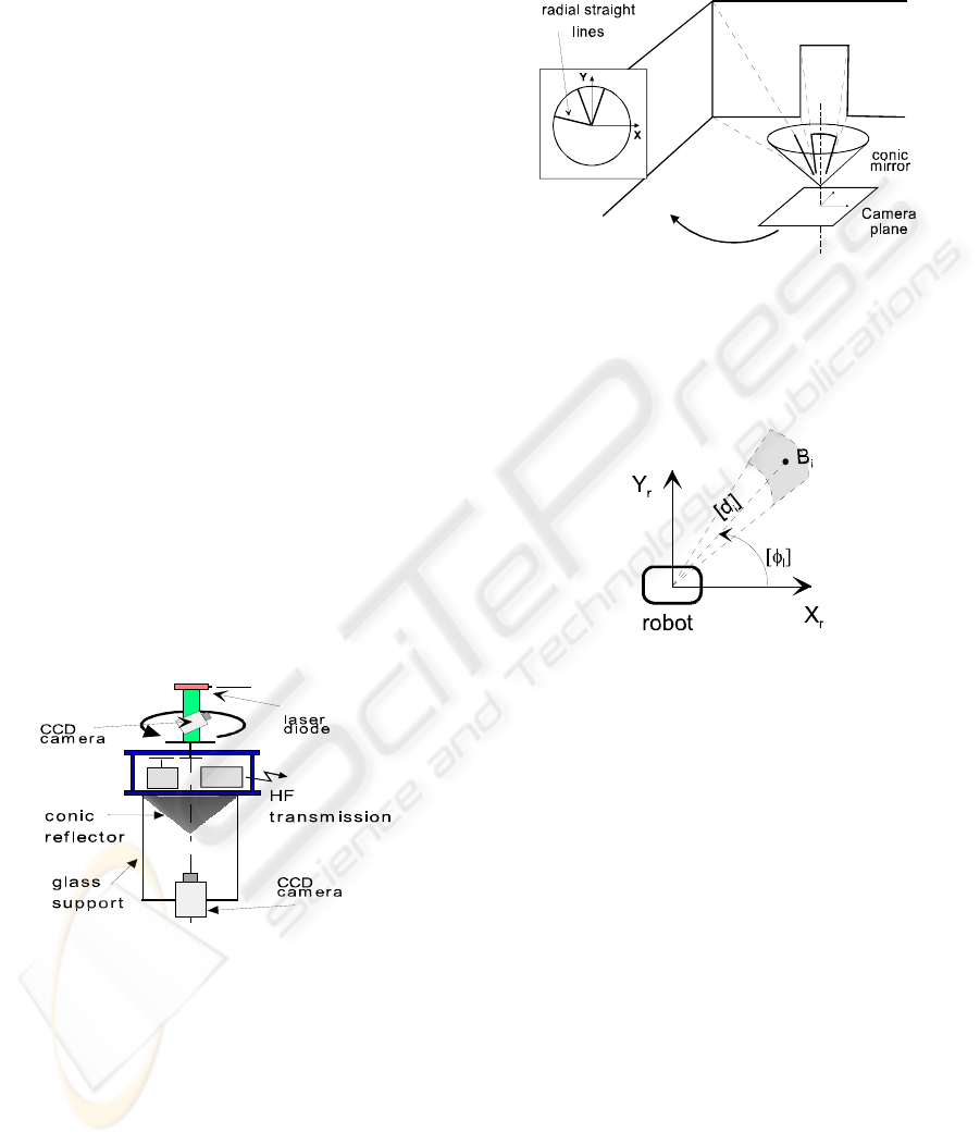
incidence angle. The SYCLOP system (Clérentin,
2001) is composed of a conic mirror and a CCD
camera. It enables us to get radial straight lines
which characterize angles of every vertical object
such as, for example, doors, corners, edges (Figure
2). These association of two sensors can be
assimilated of a depth sensor which can give a 2-D
panoramic view of the environment. See figure 2 for
an example of an experimental map.
Figure 2: Principle of the omnidirectional sensor SYCLOP
Due to the imprecision of the sensor, the polar
coordinates of the sensed primitives are expressed as
two intervals [d] and [φ], cf. Figure 3.
Figure 3: The polar coordinates of a sensed landmark Bi.
Besides, the robot is equipped with two
odometers that can give an estimate about its
position.
To localize itself, the robot has in its possession
four world maps that describe the evolution
environment: a map of segments and three maps of
high level primitives (a map of “corners”, of “edges”
and of “other primitives” ). The interest of this kind
of high level primitives is explained in (Clérentin,
2001).
The problem is to find the robot configuration q
using the exteroceptive and dead-reckoning
information. The imprecision on the sensors
measurements is modelled by intervals.
3.2 Localization principle
Our localization strategy is based on multi-target
tracking (Clérentin, 2001). The tracked primitives
are the high level primitives described before
(“corner”, “edge”, etc.). When a track is initiated,
the robot try to pursue it by matching a sensed
MOBILE ROBOT LOCALIZATION BY CONSTRAINT PROPAGATION ON INTERVALS
237

primitive with it. In our case, this multi-target
tracking can be seen as a propagation of a matching
between a theoretical primitive with sensorial
primitives during the robot displacement. Its
advantage is a lower computation time than classical
matching methods: we match a sensed primitive
only with the managed tracks at time t, not with all
the theoretical primitives.
The algorithm is then the following and will be
detailed in the next paragraphs. At each acquisition,
the robot scans its environment with the
exteroceptive sensor. It gets a map composed of
segments. Then it classifies these segments into four
classes of high level primitives: “corner”, “edge”,
“wall” and “other” (Clérentin, 2001). With the help
of the odometry information, we try to match these
primitives with one of the managed tracks. In other
words, we try to pursue the tracks. When all the
sensed primitives have been analysed, we now
consider the primitives that have not been matched
with a track and we try to associate them with a
theoretical primitive of the map in order to initiate a
new track.
3.3 Odometer modelization
Odometry is the most widely used navigation
method for mobile robot positioning. Odometry
provides good short-term accuracy, is inexpensive,
and allows very high sampling rates. The
fundamental idea of odometry is the integration of
incremental motion information over time.
Unfortunately, this leads inevitably to an
accumulation of errors. Despite this limitation, most
researchers agree that odometry is an important part
of a robot navigation system and that navigation
tasks are simplified if odometric information is
available.
The elementary displacement ∆d and elementary
rotation ∆θ of the robot are given by the following
equations:
2
rRrlRl
d
ω
ω
+
=∆
L
rRrlRl
ω
ω
θ
−
=∆
where Rl and Rr are the radius of the left and right
wheel, and ωl, ωr are the elementary rotations of the
left and right wheel.
From these equations, we can deduce from the
robot position at time n q
n
=(x
n
, y
n
, θ
n
) the
configuration at time n+1 q
n+1
=(x
n+1
, y
n+1
, θ
n+1
):
(
)
2
cos
1
θ
θ
∆
+∆+=
+ nnn dxx
(2)
(
)
2
sin
1
θ
θ
∆
+∆+=
+ nnn dyy (3)
θ
θ
θ
∆
+
=
+ nn 1 (4)
Some values involved in equations (2), (3) and
(4) are imprecise: Rl, Rr, L, ωl, ωr are not precisely
known. They are thus expressed by the way of
intervals: [Rl], [Rr], [L], [ωl], [ωr]. So the robot
configuration estimation at time n+1 given by the
odometers is now represented by a 3-D subpaving
[q
n+1
]=([x
n+1
], [y
n+1
], [θ
n+1
]), where:
[][][] []
[]
⎟
⎠
⎞
⎜
⎝
⎛
∆
+∆+=
+
2
cos
1
θ
θ
nnn dxx
(5)
[][][][]
[]
⎟
⎠
⎞
⎜
⎝
⎛
∆
+∆+=
+
2
sin
1
θ
θ
nnn dyy
(6)
[
]
[
]
[
]
θ
θ
θ
∆
+
=
+ nn 1 (7)
3.4 Initialisation of a new track
The problem is here to initiate a new track, that is to
say to match for the first time with a theoretical
primitive a sensed primitive that has not been
matched with a track. We will first argue in the case
of a primitive of type “corner”, “edge” and “other”.
We will then explain the case of a wall primitive.
Let ([d], [φ]) be the imprecise coordinates
(expressed by intervals) of the junction point of a
“corner”, “edge” or “other” primitive (see Figure 4
for the case of a corner). Let [q
n+1
]=([x
n+1
], [y
n+1
],
[θ
n+1
]) be the robot configuration estimation given
by the odometry. With this estimation, we can
compute the Cartesian coordinates ([x], [y]) of the
sensed landmark in the world reference frame (Xe,
Ye):
][])[]cos([][][ 11 ++ +
+
×
=
nn xdx
θ
φ
(8)
][])[]sin([][][ 11 ++ +
+
×
=
nn ydy
θ
φ
(9)
ICINCO 2004 - ROBOTICS AND AUTOMATION
238
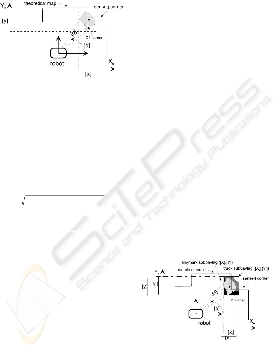
Figure 4: A corner primitive case: the theoretical corner
C1 is candidate for a matching.
With this result, the association method is quite
simple: a new track is initialised if a theoretical
landmark of the same type is included in the
subpaving ([x], [y]). For example, on figure 4, the
theoretical corner C1 is candidate for a matching
since its Cartesian coordinates are included in ([x],
[y]).
When a theoretical candidate whose coordinates
are (x
theo
, y
theo
) is found, the resulting matching links
the polar coordinates of the sensed landmark ([d],
[φ]) with the robot position estimation [q
n+1
]=([x
n+1
],
[y
n+1
], [θ
n+1
]) through these two equations :
[]
()
[]
()
2
1
2
1
][ theontheon yyxxd −+−= ++
(10)
[]
()
[]
()
[]
1
1
1
arctan][ +
+
+
−
−
−
= n
ntheo
ntheo
xx
yy
θφ
(11)
These two equations (10) and (11) implies two
new constraints on the robot position estimation
[q
n+1
]=([x
n+1
], [y
n+1
], [θ
n+1
]) given by constraints (5),
(6) and (7). So we have to solve a CSP by using the
forward backward propagation algorithm explained
on paragraph 2.2. Naturally, the constraints (10) and
(11) reduce the size of the subpaving of the robot
configuration [q
n+1
]. In other words, they decrease
the localization imprecision.
This propagation can give a non-valid solution,
that is to say there is no solution for the CSP because
all the values are inconsistent. This means that the
theoretical landmark that has been selected for the
matching is not valid, so it is rejected. In this case,
the algorithm is eventually restarted with an other
theoretical landmark which is included on the
subpaving ([x], [y]). If there is no other theoretical
candidate, the sensed landmark is considered as an
outlier.
The initialisation of “wall” track is performed as
the same way, except that we have to consider two
coordinates : the two wall endpoints.
This algorithm is performed on each sensed
primitive which is not associated to any track. At
each new initialisation, the localization imprecision,
i.e. the robot configuration subpaving, is reduced
thanks to the CSP solving.
So, at the end of this stage, we have several new
tracks that are characterized by the subpaving ([x],
[y]) which permitted to initialise them. Let call this
subpaving the “track subpaving”.
3.5 Propagation of a track
In this part, we try to propagate the matchings
initialised in the previous paragraph with the
observations made during the robot’s displacement.
In other words, we try to associate tracks with
sensed landmarks.
Suppose we manage q tracks at time n. Each
track is characterized by its “track subpaving”
(expressed in the world reference frame). Let call
this track suppaving ([x
t
], [y
t
]). Suppose the robot
gets p observations at time n+1. As we have
explained in paragraph 3.4, we are able to compute
each observation localization subpaving ([x], [y]) in
the world reference frame thanks to the equations (8)
and (9). So, for each track, we have to search among
the p sensed primitives the one that corresponds to
the track. In other word, we have to match a track
subpaving ([x
t
], [y
t
]) with an observation subpaving
([x], [y]), cf. figure 5. The matching criterion we
choose is based on the percentage of overlapping
between these two kinds of subpaving ([x
t
], [y
t
]) and
([x], [y]) in comparison with the size of the track
subpaving.
Figure 5: The track propagation principle in a corner
primitive case.
So at this level, the problem is to match for each
type of primitive the p observations obtained at the
MOBILE ROBOT LOCALIZATION BY CONSTRAINT PROPAGATION ON INTERVALS
239
acquisition n+1 with the q tracks. To reach this aim,
we use the Transferable Belief Model (Smets, 1998)
in the framework of extended open word (Royère,
2002) because of the introduction in the frame of
discernment of an element noted * which represents
all the hypothesis which are not modelled.
For each track Qj (j ∈ [1..q]), we apply the
following algorithm:
– The frame of discernment Θ is composed of:
– the p observations represented by the hypothesis
Pi (i ∈ [1..p]). Pi means “the track Qj is matched
with the observation Pi”)
– and the element * which means “the track Qj
cannot be matched with one of the p
observations”.
So: Θ={P
1
, P
2
, …, *}
– The matching criterion is the overlapping
percentage between the subpaving of observation
Pi and the track subpaving of Qj (Figure 6)
– Considering the basic probability assignment
(BPA) shown figure 6, we compute for each
observation Pi:
– m
i
(Pi) the mass associated with the proposition
“Pi is matched with Qj”.
– m
i
(¬Pi) the mass associated with the proposition
“Pi is not matched with Qj”.
– m
i
(Θ) the mass represented the ignorance
concerning the observation Pi.
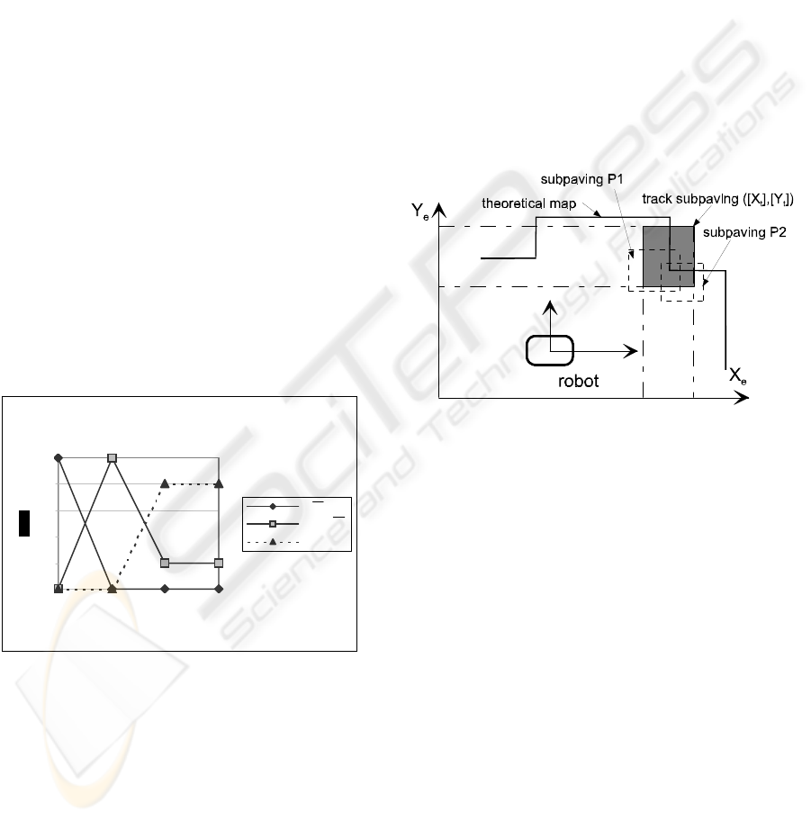
The BPA is shown on Figure 6.
Overlapping percentage
0
0,2
0,4
0,6
0,8
1
025100150
percent age
m(Pi)
m(Pi U Pi)
m(Pi)
Figure 6: BPA of the matching criterion.
– After the treatment of all the Pi observations, we
have p triplets :
m
1
(P
1
) m
1
(¬P
1
) m
1
(Θ)
m
2
(P
2
) m
2
(¬P
2
) m
2
(Θ)
…
m
p
(P
p
) m
p
(¬P
p
) m
p
(Θ)
We fuse these triplets using the disjunctive
conjunctive operator built by Royère (Royère,
2002). Indeed, this operator allows a natural
conflict management, ideally adapted for our
problem. In our case, the conflict comes from the
existence of several potential candidates for the
matching, that is to say some near sensed
landmarks can correspond to a track. With this
operator, the conflict is distributed on the union
of the hypothesis which generate this conflict.
For example, on figure 7, the subpavings P
1
and
P
2
are candidate for a matching with the track
subpaving ([x
t
], [y
t
]). So m
1
(P
1
) is high (the
expert concerning P
1
says that P
1
can be match
with ([x
t
], [y
t
])) and m
2
(P
2
) is high too. If the
fusion is performed with the classical Dempster
operator, these two high values produce a high
conflict. But, with the Royère operator, the
conflict generated by m
1
(P
1
) and m
2
(P
2
) is
rejected on m
12
(P
1
∪ P
2
). This means that both
P
1
and P
2
are candidate for the matching.
Figure 7: An example of two landmark subpavings that
generate some conflict.
– So, after the fusion of the p triplets with the
Royere operator, we get a mass on all single
hypothesis m
match
(Pi), on all the unions of
hypothesis m
match
(Pi ∪ Pj…∪ Pk), on the star
hypothesis m
match
(*) and on the ignorance
m
match
(Θ).
– The final decision is the hypothesis which has
the maximal pignistic probability (Smets, 1998).
If it is the * hypothesis, no matching is achieved.
This case corresponds to temporary or definitive
disappearance of the track, due to a temporary or
complete occultation of the primitive.
Once a matching is achieved, the method is like the
initialisation step (paragraph 3.4): the robot position
and the track, that is to say a theoretical landmark,
are linked by the polar coordinates ([d], [φ]) of the
sensed landmark. Therefore, these considerations
imply the same two constraints given by the
equations (10) and (11) on the robot localization
ICINCO 2004 - ROBOTICS AND AUTOMATION
240
estimation given by equations (5), (6) and (7). These
equations form a CSP we solve by using the forward
backward propagation algorithm explained on
paragraph 2.2.
When this propagation has no solution, the
matching is cancelled and the relative observation
could be used to an other matching, for pursuit or for
initialisation.
3.6 Summary of the localization
method
Let resume our localization paradigm. When the
robot has done a sensorial acquisition, the multi
target tracking algorithm explained on paragraph 3.5
is performed for each existing tracks. Then, all the
sensed primitives that have not been matched with
any tracks are used to initialise new tracks, as
explained in paragraph 3.4.
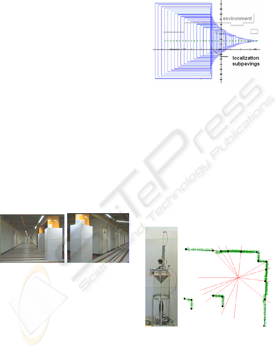
4 EXPERIMENTAL RESULTS
In this part, we present the experimental results we
obtained after several acquisitions in an indoor
environment (the end of a corridor shown figure 8).
The mobile robot execute two paths composed of
forty-six acquisitions made every 30 cm and
computed in a Pentium PC located on the robot.
Figure 8: The experimental environment.
On figure 9, we show the 3D localisation
subpavings of the robot obtained using only the
odometric information. We can note the classical
phenomena of cumulative error: the size of the
subpavings increases unceasingly. This shows the
need to add to dead reckoning the measurements
given by an other sensor.
Figure 9: Localization results using only odometry.
An example of sensed map obtained with our
omnidirectional sensor with associates the SYCLOP
sensor and a telemeter is shown on figure 10. The
crosses represent the depth points given by the
telemeter. The red lines on the centre of the figure
are the radial straight lines issued of the treatment of
the SYCLOP image. Finally, a segmentation stage
gives us a set of segments (the black ones on figure
10).
The experimental results using dead reckoning
and the depth sensor are shown on figure 11. The
true localizations are represented by the black
points. Firstly, we note a relatively precise
localization: the localization subpavings have a
small size (lower than 20 cm in X and Y, and 11
degrees in orientation). The error is weak (10 cm in
position and one degree in orientation).
Figure 10: the perception system and an example of high
level primitive map.
MOBILE ROBOT LOCALIZATION BY CONSTRAINT PROPAGATION ON INTERVALS
241
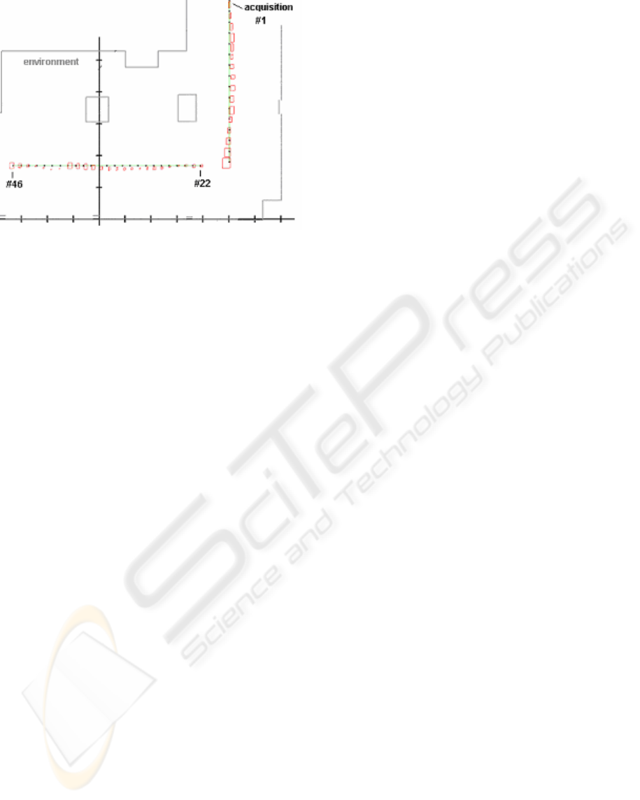
Figure 11: two dimensions localization results.
5 CONCLUSION
We have presented in this article a localization
method based on constraint propagation on intervals.
Indeed, the localization problem can be modelled as
a constraint satisfaction problem (CSP). In our case,
the imprecise information used to localize the robot
come from two sensors: two odometers and an
exteroceptive sensor. These two sensors give
measurements which are linked by some constraints.
These constraints induce a reduction of the
subpaving which represents the robot localization.
Another advantage of this method is its ability to
treat naturally and easily imprecise data: these data
are represented by intervals. So, the localization
imprecision quantification is intrinsically managed
by our algorithm.
The localization strategy is based on multi target
tracking. This strategy, which can be seen in our
case as a propagation of a matching during the
robot’s displacement, is less complex than classical
methods. Besides, our matching method, which is
based on the use of the TBM, gives us an uncertainty
value about each matching done. This value can
allow to estimate an uncertainty about each track,
and thus manage the problem of track cancel: if a
track is to uncertain, it will be cancelled. This track
uncertainty management is one of the main future
perspectives that will concern this work.
REFERENCES
Smets, Ph, 1998. The Transferable Belief Model for
Quantified Belief Representation, Handbook of
Defeasible Reasoning and Uncertainty Management
Systems, Kluwer Ed, pp 267-301.
Jaulin L, Braems I, Kieffer M, Walter E, 2001. Nonlinear
state estimation using forward-backward propagation
of intervals in an algorithm, In Scientific Computing,
Validated Numerics, Interval Methods, pp191-204,
Kluwer Academic Publishers.
Moore R.E, 1979. Methods and applications of interval
analysis, SIAM, Philadelphia.
Jaulin L, Kieffer M, Didrit O, Walter E, 2001. Applied
interval analysis, Springer-Verlag
Leonard J, Durrant-Whyte H, 1991. Mobile robot
localization by tracking geometric beacons, IEEE
Trans. on Robotics and Automation, Vol. 7, n°3, pp.
89-97.
Chung H, Ojeda L, Borenstein J, 2001. Sensor fusion for
Mobile Robot Dead-reckoning With a Precision-
calibrated Fiber Optic Gyroscope – proc. of the 2001
IEEE Int. Conf. on Robotics & Automation, pp.3588-
3593.
Bouron P, Meizel D, Bonnifait P, 2001. Set-membership
non-linear observers with application to vehicle
localisation, ECC'01 European Control Conference.
Clerentin A, Delahoche L, Brassart E, 2001.
Omnidirectional sensors cooperation for multi-target
tracking, IEEE Int . Conf. on Multisensor Fusion and
Integration for Intelligent Systems (MFI 2001).
Clerentin A, Delahoche L, Brassart E, Cauchois C, 2002.
An Uncertainty Propagation Architecture for the
Localization Problem, Workshop on Performance
Metrics for Intelligent Systems PerMIS2002, NIST,
Washington, USA, August 2002
Royere C, 2002. Contribution à la résolution du conflit
dans le cadre de la théorie de l’évidence, PhD thesis,
Université de Technologie de Compiègne, 2002
Clerentin A, Delahoche L, Brassart E, Drocourt C, 2003..
Uncertainty and error treatment in a dynamic
localization system, proc. of the 11th Int. Conf. on
Advanced Robotics (ICAR03), pp.1314-1319,
Coimbra, Portugal.
Preciado A, Meizel D, Segovia A, Rombaut M, 1991.
Fusion of multi-sensor data: a geometric approach”, in
proc. IEEE Int. Conf. On Robotics and Automation
(ICRA’91), vol 3, pp. 2806-2811, Sacramento, USA.
Hanebeck U.D, Schmidt G, 1996. Set theoretic
localization of fast mobile robots using an angle
measurement technique, in proc. IEEE Int. Conf. On
Robotics and Automation (ICRA’96), pp. 1387-1394.
Meizel D, Leveque 0, Jaulin L, Walter E, 2002. Initial
Localization by Set Inversion. IEEE trans. on Robotics
and Automation. Vol 18, n° 6, pp 966-971.
ICINCO 2004 - ROBOTICS AND AUTOMATION
242
