
MODEL PREDICTIVE CONTROL FOR HYBRID SYSTEMS
UNDER A STATE PARTITION BASED MLD APPROACH
(SPMLD)
Jean Thomas, Didier Dumur
Supélec, F 91192 Gif sur Yvette cedex, France
Jean Buisson, Herve Guéguen
Supélec, F 35 511 Cesson-Sévigné cedex, France
Keywords: Hybrid dynamical systems, Mixed Logical Dynamical systems (MLD), Piecewise Affine systems (PWA),
Model Predictive Control (MPC)
Abstract This paper presents the State Partition based Mixed
Logical Dynamical (SPMLD) formalism as a new
modeling technique for a class of discrete-time hybrid systems, where the system is defined by different
modes with continuous and logical control inputs and state variables, each model subject to linear
constraints. The reformulation of the predictive strategy for hybrid systems under the SPMLD approach is
then developed. This technique enables to considerably reduce the computation time (with respect to the
classical MPC approaches for PWA and MLD models), as a positive feature for real time implementation.
This strategy is applied in simulation to the control of a three tanks benchmark.
1 INTRODUCTION
Hybrid systems become an attractive field of
research for engineers as it appears in many control
applications in industry. They include both continu-
ous and discrete variables, discrete variables coming
from parts described by logic such as for example
on/off switches or valves. Various approaches have
been proposed for modeling hybrid systems (Brani-
cky et al., 1998), like Automata, Petri nets, Linear
Complementary (LC), Piecewise Affine (PWA)
(Sontag, 1981), Mixed Logical Dynamical (MLD)
models (Bemporad, and Morari, 1999).
This paper examines a class of discrete-time
hy
b
rid systems, which consists of several models
with different dynamics according to the feasible
state space partition. Each model is described with
continuous and logical states and control inputs.
Consequently, the dynamic of the system depends
on the model selected in relation to linear constraints
over the states and on the inputs values.
On the other hand, model predictive control
(MPC) appea
r
s to be an efficient strategy to control
hybrid systems. Considering the previous particular
class of hybrid systems, implementing MPC leads to
a problem including at each prediction step the states
and inputs vectors (both continuous and discrete
variables), the dynamic equation and linear
constraints, for which a quadratic cost function has
to be optimized. Two classical approaches exist for
solving this optimization problem.
First, all possible logical combinations can be
studie
d
at each prediction time, which leads solving
a great number of QPs. Each of these QPs is related
to a particular scenario of logical inputs and modes.
This is the PWA approach. The number of QPs can
be reduced by reachability considerations (Pena et
al., 2003).
The second moves the initial problem through
th
e MLD fo
rmalism to a single general model used
at each prediction step. This MLD formalism
introduces many auxiliary logical and continuous
variables and linear constraints. At each prediction
step, all the MLD model variables have to be solved
(even if some of them are not active). However, the
MLD transformation allows utilizing the Branch and
Bound (B&B) technique (Fletcher and Leyffer,
1995), reducing the number of QPs solved.
This paper develops a technique which aims at
im
ple
menting MPC strategy for the considered class
of hybrid systems, as a mixed solution of the two
classical structures presented before. It is based on a
78
Thomas J., Dumur D., Buisson J. and Guéguen H. (2004).
MODEL PREDICTIVE CONTROL FOR HYBRID SYSTEMS UNDER A STATE PARTITION BASED MLD APPROACH (SPMLD).
In Proceedings of the First International Conference on Informatics in Control, Automation and Robotics, pages 78-85
DOI: 10.5220/0001137000780085
Copyright
c
SciTePress
new modeling technique, called State Partition based
MLD approach (SPMLD) formalism, combining the
PWA and MLD models. The complexity of this
formalism is compared to that obtained with the
usual PWA and MLD forms, which can also model
this class of hybrid systems as well.
The paper is organized as follows. Section 2
presents a short description of the PWA and MLD
hybrid systems. General consideration about model
predictive control (MPC) and its classical
application to PWA and MLD systems are
summarized in Section 3. Section 4 develops the
State Partition based MLD approach (SPMLD) and
examines the application of MPC to hybrid systems
under this formalism. Section 5 gives an application
of this strategy to water level control of a three tanks
benchmark. Section 6 gives final conclusions.
2 HYBRID SYSTEMS MODELING
2.1 Mixed Logical Dynamical model
The MLD model appears as a suitable formalism for
various classes of hybrid systems, like linear hybrid
or constrained linear systems. It describes the sys-
tems by linear dynamic equations subject to linear
inequalities involving real and integer variables,
under the form (Bemporad and Morari, 1999)
(1)
54132
321
3211
ExEuEzEδE
zDδDuDCxy
zBδBuBAxx
++≤+
+++=
+++=
+
kkkk
kkkkk
kkkkk
where
{}
l
c
n
n
l
c
1,0×ℜ∈
⎟
⎟
⎠
⎞
⎜
⎜
⎝
⎛
=
x
x
x , ,
{}
l
c
m
m
l
c
1,0×ℜ∈
⎟
⎟
⎠
⎞
⎜
⎜
⎝
⎛
=
u
u
u
{}
l
c
p
p
l
c
1,0×ℜ∈
⎟
⎟
⎠
⎞
⎜
⎜
⎝
⎛
=
y
y
y , ,
{}
l
r
1,0∈δ
c
r
ℜ∈z
are respectively the vectors of continuous and binary
states of the system, of continuous and binary
(on/off) control inputs, of output signals, of auxiliary
binary and continuous variables.
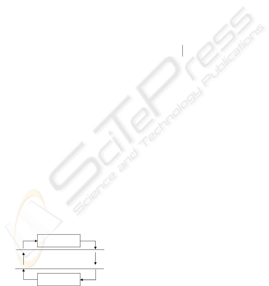
Discrete/ Digital
Continuous dynamic
system
D/A
A/D
0 else
1
if
=
=
≤
δ
δ
bax
22
11
else
1 if
bxaz
bxaz
+=
+=
=
δ
Figure 1: MLD model structure
The auxiliary variables are introduced when
translating propositional logic into linear inequalities
as described in Figure 1. All matrices appearing in
(1) can be obtained through the specification
language HYSDEL (Hybrid System Description
Language), see (Torrisi et al., 2000).
2.2 Piecewise Affine model
Another framework for discrete time hybrid systems
is the PWA model (Sontag, 1981), defined as
⎪
⎭
⎪
⎬
⎫
⎪
⎩
⎪
⎨
⎧
+=
++=
+
i
k
i
k
i
k
i
k
i
k
i
S
gxCy
fuBxAx
1
: , for: (2)
i
k
k
χ
∈
⎥
⎦
⎤
⎢
⎣
⎡
u
x
where
{
}
s
i
i
1=
is the polyhedral partition of the state
and input spaces (s being the number of subsystems
within the partition). Each
χ
i
χ
is given by
⎪
⎭
⎪
⎬
⎫
⎪
⎩
⎪
⎨
⎧
≤
⎥
⎦
⎤
⎢
⎣
⎡
⎥
⎦
⎤
⎢
⎣
⎡
=
i
k
k
i
k
k
i
q
u
x
Q
u
x
χ
(3)
where
kkk
denote the state, input and output
vector respectively at instant
. Each subsystem
i
defined by the 7-uple
yux ,,
k S
(
)
,,,,,,,
iiiiiii
qQgfCBA
(
)
si ,,2,1 L
∈
is a component of the PWA system
(2).
(
)
mnp
inpimninni
i
+
×××
ℜ∈ℜ∈ℜ∈ℜ∈ QCBA ,,,
and
are suitable constant vectors or
matrices, where
, , are respectively the
number of states, inputs, outputs, and
i
is the
number of hyperplanes defining the
i -polyhedral. In
this formalism, a logical control input is considered
by developing an affine model for each input value
(1/0), defining linear inequality constraints linking
the model with the relevant input value.
iii
qgf ,,
n m
p
p
It has been shown in (Bemporad et al., 2000),
that MLD and PWA models are equivalent, which
enables transformation from one model to the other.
A MLD model can be transferred to a PWA model
with the number of subsystems inside the polyhedral
partition equal to all possible combination of all the
integer variables of the MLD model (Bemporad et
al., 2000) (a technique for avoiding empty region is
presented in (Bemporad, 2003))
(4)
lll
rmn
s
++
= 2
3 MODEL PREDICTIVE CONTROL
Model predictive control (MPC) has proved to
efficiently control a wide range of applications in
industry, including systems with long delay times,
non-minimum phase, unstable, multivariable and
constrained systems.
The main idea of predictive control is the use of
a plant model to predict future outputs of the system.
Based on this prediction, at each sampling period, a
sequence of future control values is elaborated
MODEL PREDICTIVE CONTROL FOR HYBRID SYSTEMS UNDER A STATE PARTITION BASED MLD
APPROACH (SPMLD)
79

through an on-line optimization process, which
maximizes the tracking performance while satisfying
constraints. Only the first value of this optimal
sequence is applied to the plant according to the
‘receding’ horizon strategy (Dumur and Boucher,
1998).
Considering the particular class of hybrid
systems previously described, implementing MPC
leads to a problem including at each prediction step
the states vector, the inputs vector (both continuous
and discrete), the dynamic equation and linear
constraints, for which a quadratic cost function has
to be optimized. Two classical approaches exist for
solving this optimization problem, the Branch and
Bound technique that can be used with the MLD
formalism and the enumeration of all possible
logical system combinations at each prediction time
corresponding to all particular scenarios of logical
inputs and modes used with the PWA formalism.
3.1 Model predictive control for the
MLD systems
For a MLD system of the form (1), the following
model predictive control problem is considered. Let
be the current time,
k
the current state,
an equilibrium pair or a reference
trajectory value,
the final time, find
k
the sequence which
moves the state from
to and minimizes
k x
),(
ee
ux
Nk +
(
1
1
−+
−+
=
Nkk
Nk
)
uuu L
k
x
e
x
2
/
2
/1
2
/
2
/
1
0
2
1
54
32
1
1
),(min
QQ
QQ
Q
yyxx
zzδδ
uxu
u
ekikekik
ekikekik
N
i
eikk
Nk
k
uJ
Nk
k
−+−+
+−+−+
+−=
+++
++
−
=
+
−+
∑
−+
(5)
subject to (1), where
is the prediction horizon,
e
,
e
are the auxiliary variables of the equilibrium
point or the reference trajectory value, calculated by
solving a MILP problem for the inequality equation
of (1).
ki
denotes the predicted state vector at
time
, obtained by applying the input sequence
to model (1) starting from the current state
(same for the other input and output variables),
, , and
'
, for
.
N
δ z
k /+
x
ik +
1−+Nk
'
≥=
ii
QQ
k
u
k
x
0>=
ii
QQ
4,1for =i
0
5,3,2 =i
The optimization procedure of (5) leads to MIQP
problems with the following optimization vector
(6)
T
1
11
],,,
,,,,,,[
−+
−+−+
=
Nkk
NkkNkk
zz
δδuuχ
L
LL
The number of binary optimization variables is
(
)
ll
rmNL
+
=
. In the worst case, the maximum
number of solved QP problems is
No of QPs
12
1
−
=
+L
(7)
So the main drawback of this MLD formalism
remains the computational burden related to the
complexity of the derived Mixed Integer Quadratic
Programming (MIQPs) problems. Indeed MIQPs
problems are classified as NP-complete, so that in
the worst case, the optimization time grows expo-
nentially with the problem size, even if branch and
bounds methods (B&B) may reduce this solution
time (Fletcher and Leyffer, 1995).
3.2 Model Predictive control for the
PWA systems
Considering the PWA system under the form (2),
assuming that the current state
k
is known the
model predictive control requires solving at each
time step (Pena et al., 2003).
x
maxmin
1
0
2
1
2
/
1
:s.t.
),(min
1
uuu
u
wyxu
u
≤≤
+
−=
+
−
=
+
=
++
−+
∑
∑
−+
ik
N
i
ikii
N
i
ikkikiik
Nk
k
r
qJ
Nk
k
(8)
where
is the prediction horizon,
ik+
is the
output reference, and
ki
denotes the predicted
output vector at time
N w
k /+
y
ik
+
, obtained by applying the
input sequence
k
u
to the
system starting from the current state
k
.
iiii
are
the elements of
weighting diagonal matrices.
()
1
1
−+
−+
=
Nkk
Nk
uu L
x rq ,
RQ,
In order to solve this equation the model applied
at each instant has to be determined and all potential
sequences of subsystems
have to be examined, where
ik
is one sub-region
among the s subsystems at prediction time
i
for
{}
11
,,,
−++
=
Nkkk
IIII L
I
+
1,,2,1
−
=
Ni L
. As for each model the value of the
logical variable is fixed, the MPC problem is solved
by a QP for each potential sequence. As the current
state
k
is known, the starting region according to
the state partition is identified. But the initial sub-
region related to the current input control is not
known as it appears in the domain definition (3).
Similarly, the next steps subsystems are also
unknown, depending on the applied control
sequence. In general, all potential sequences of
subsystems
x
I
have to be examined, which increases
the computation burden. If no constraints are
considered, the number of possible sequences for a
prediction horizon
is , where
p
is the
number of all possible sub-regions at instant
N
1−N
p
sm
m
k
ICINCO 2004 - SIGNAL PROCESSING, SYSTEMS MODELING AND CONTROL
80

according to the input space partition. In order to
solve the MPC problem of (8), the number of
quadratic programming problems to be solved is
No QPs
(9)
1−
=
N
p
sm
4 MPC FOR STATE PARTITION
BASED MLD (SPMLD)
FORMALISM
4.1 The SPMLD formalism
The SPMLD model is a mixed approach where in
each region of the feasible space a simple MLD
model is developed. Starting from the MLD model,
the auxiliary binary variables are divided into two
groups
. Where is
chosen in order to include the
[
21
δδδ =
]
T r
{}
2
1,0
2
l
∈δ
δ
variables that are
not directly depending on the state variables (the
inequalities that define
δ
variables are not
depending on
x ), and depending on .
This partition will be further justified. The SPMLD
model is then developed by giving
1
δ a constant
value: for each possible combination of
1
δ a sub-
region is defined with the corresponding
i
constraints as in (3). As some logical combinations
may not be feasible, the number of sub-regions of
the polyhedral partition is
{}
1
1,0
1
l
∈δ
r
i
0
)(
δ
δ
xf
zxfz
,,,, EDCBA
ii
,, EDC
x
qQ ,
(10)
1
2
l
r
s ≤
Consequently, this model requires a smaller number
of sub-regions than the classical PWA model for the
same modeled system. Each sub-region has its own
dynamic described in the same way as (1) but with a
simpler MLD model that represents the system
behavior in this sub-region and includes only the
active variables in this sub-region. This partition
always implies a reduction in the size of
and/or
. For example, some control variables may not be
active in sub-regions and the auxiliary continuous
variables
depending on the
1
δ variables may
disappear or become fixed as
is fixed where:
z
u
z
1
δ
(11)
⎩
⎨
⎧
=
=
=→=
1 if)(
0 if
δ
Consequently, simplified sub-regions models can be
derived, an example of this simplification is given in
the application section.
The system is thus globally modeled as
(12)
i
k
i
k
i
k
i
k
i
k
i
k
i
k
i
k
i
k
k
i
k
i
k
i
k
i
k
54132
321
3211
ExEuEzEδE
zDδDuDxCy
zBδBuBxAx
++≤+
+++=
+++=
+
iiiii
513131
−−−
are the matrices of the i
th
MLD model defining the dynamics into that sub-
region.
constraints has to be included in (12). qQ ,
4.2 Reformulation of the MPC solution
At this stage, the MPC technique developed for the
PWA formalism must be rewritten to fit the new
SPMLD model. Consider the initial subsystem
k
I
(13)
k
k
k
k
k
k
k
k
k
k
k
k
k
k
k
k
k
k
zDδDuDxCy
zBδBuBxAx
321
321
1
+++=
+++=
+
with
k
kk
k
k
k
k
k
k
δEExEzEuE
2
5
431
−+≤+−
Where
will now denote for simplification
purposes the
matrix of model i at instant (the
same notations are used for
B
).
k
A
i
A
k
kkkk
513131
−−−
For a given sequence over the prediction horizon
i.e. for
,
N
{
}
11
,,,
−++
=
Nkkk
IIII L , the system is
recursively defined as follows
zGδPuHxFy
zGδPuHxFx
yyyky
xxxkx
+++=
+++=
(14)
Where
[
]
,
T
21 Nkkk +++
= xxxx L
[
]
[
]
T
1
T
1
,
−+−+
==
NkkNkk
yyyuuu LL
[
]
[
]
T
1
T
1
,
−+−+
==
NkkNkk
δδδzzz LL
⎥
⎥
⎥
⎥
⎥
⎦
⎤
⎢
⎢
⎢
⎢
⎢
⎣
⎡
=
⎥
⎥
⎥
⎥
⎥
⎦
⎤
⎢
⎢
⎢
⎢
⎢
⎣
⎡
=
−+−+
+
−+
+
kNkNk
kk
k
kNk
kk
k
AAC
AC
C
F
AA
AA
A
F
yx
L
M
L
M
21
1
1
1
,
⎥
⎥
⎥
⎥
⎥
⎦
⎤
⎢
⎢
⎢
⎢
⎢
⎣
⎡
=
−+++−++−+
++
1
1
1
1
21
1
11
1
11
1
1
0
00
NkkkNkkkNk
kkk
k
BBAABAA
BBA
B
H
x
LLL
MOMM
L
L
⎥
⎥
⎥
⎥
⎥
⎦
⎤
⎢
⎢
⎢
⎢
⎢
⎣
⎡
=
−+++−++−+
++
1
3
1
3
21
3
11
1
33
1
3
0
00
NkkkNkkkNk
kkk
k
BBAABAA
BBA
B
G
x
LLL
MOMM
L
L
⎥
⎥
⎥
⎥
⎥
⎦
⎤
⎢
⎢
⎢
⎢
⎢
⎣
⎡
=
−+++−++−+
++
1
2
1
2
21
2
11
1
22
1
2
0
00
NkkkNkkkNk
kkk
k
BBAABAA
BBA
B
P
x
LLL
MOMM
L
L
⎥
⎥
⎥
⎥
⎥
⎦
⎤
⎢
⎢
⎢
⎢
⎢
⎣
⎡
=
−+++−+−++−+−+
++
1
1
1
1
221
1
121
1
11
1
1
0
00
NkkkNkNkkkNkNk
kkk
k
DBAACBAAC
DBC
D
H
y
LLL
MOMM
L
L
⎥
⎥
⎥
⎥
⎥
⎦
⎤
⎢
⎢
⎢
⎢
⎢
⎣
⎡
=
−+++−+−++−+−+
++
1
3
1
3
221
3
121
1
33
1
3
0
00
NkkkNkNkkkNkNk
kkk
k
DBAACBAAC
DBC
D
G
y
LLL
MOMM
L
L
MODEL PREDICTIVE CONTROL FOR HYBRID SYSTEMS UNDER A STATE PARTITION BASED MLD
APPROACH (SPMLD)
81

⎥
⎥
⎥
⎥
⎥
⎦
⎤
⎢
⎢
⎢
⎢
⎢
⎣
⎡
=
−+++−+−++−+−+
++
1
2
1
2
221
2
121
1
22
1
2
0
00
NkkkNkNkkkNkNk
kkk
k
DBAACBAAC
DBC
D
P
y
LLL
MOMM
L
L
Then the MPC optimization problem (8) leads to the
following cost function
[]
ooo
g
δ
z
u
f
δ
z
u
HδzuJ +
⎥
⎥
⎥
⎦
⎤
⎢
⎢
⎢
⎣
⎡
+
⎥
⎥
⎥
⎦
⎤
⎢
⎢
⎢
⎣
⎡
= 2
(15)
where
⎥
⎥
⎥
⎥
⎥
⎦
⎤
⎢
⎢
⎢
⎢
⎢
⎣
⎡
+
=
y
T
y
T
y
T
y
T
y
T
y
T
y
T
y
T
y
T
o
yyy
yyy
yyy
PQPGQPHQP
PQGGQGHQG
PQHGQHRHQH
H
T
y
T
y
T
y
T
k
y
T
y
T
y
T
k
y
T
y
T
y
T
k
o
⎥
⎥
⎥
⎥
⎦
⎤
⎢
⎢
⎢
⎢
⎣
⎡
−
−
−
=
PQwPQFx
GQwGQFx
HQwHQFx
f
]2[ wQwxFQwxFQFxg
T
ky
T
ky
T
y
T
ko
+−=
[]
(
)
[]
()
0,diag
0,diag
f
f
T
ii
T
ii
q
r
QQQ
RRR
==
==
This technique allows choosing different weighting
factors for each sub-region according to its priority.
The constraints over the state and input domains
for each sub-region are included in the inequality
equation of the MLD model of that sub-region using
the HYSDEL program. The MPC optimization
problem (15) is solved subject to the constraints
[]
N
δ
z
u
MMM ≤
⎥
⎥
⎥
⎦
⎤
⎢
⎢
⎢
⎣
⎡
231
(16)
where
⎥
⎥
⎥
⎥
⎥
⎦
⎤
⎢
⎢
⎢
⎢
⎢
⎣
⎡
+
+
+
=
−+−+−+
++
1
5
21
4
1
5
1
4
54
Nk
k
kNkNk
k
k
kk
k
k
k
ExAAE
ExAE
ExE
N
L
M
⎥
⎥
⎥
⎥
⎥
⎦
⎤
⎢
⎢
⎢
⎢
⎢
⎣
⎡
−−−
−−
−
=
−+++−+−++−+−+
++
1
1
1
1
221
41
121
4
1
11
1
4
1
1
0
0
00
NkkkNkNkkkNkNk
kkk
k
EBAAEBAAE
EBE
E
M
LLL
OMM
L
L
⎥
⎥
⎥
⎥
⎥
⎦
⎤
⎢
⎢
⎢
⎢
⎢
⎣
⎡
−−
−
=
−+−+−++−+−+
++
1
2
2
2
1
42
121
4
1
22
1
4
2
2
0
0
00
NkNkNkkkNkNk
kkk
k
EBEBAAE
EBE
E
M
LL
OMM
L
L
⎥
⎥
⎥
⎥
⎥
⎦
⎤
⎢
⎢
⎢
⎢
⎢
⎣
⎡
−−
−
=
−+−+−++−+−+
++
1
3
2
3
1
43
121
4
1
33
1
4
3
3
0
0
00
NkNkNkkkNkNk
kkk
k
EBEBAAE
EBE
E
M
LL
OMM
L
L
The number of binary optimization variables, with
known and constant, is given by the relation
1
δ
(17)
{
sjrmL
N
i
i
jl
i
lj
,,2,1,
1
0
2
L∈+=
∑
−
=
}
rm ,
δ
Where
lj
are the number of modeled logical
control and
2
elements respectively in the j
i
jl
i
2
th
sub-
region at prediction time
i
.
Therefore, if the sequence
I
is fixed, the
problem can be solved minimizing (15) subject to
the constraints of (16). But, as only
k
is known
(where
is considered as known, and
depends on ), all possible sequences as in
Figure 2 have to be solved. So the number of
possible sequences is
. The optimal solution is
provided by the resolution of these
MIQPs. In
order to find the solution more quickly, these
problems are not solved independently and the
optimal value of the criterion provided by the solved
MIQP is used to bind the result of the others. It can
then be used by the B&B algorithm to cut branches.
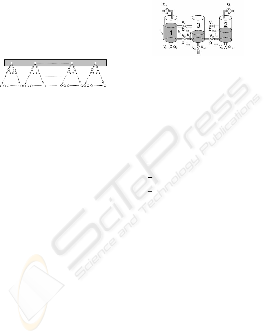
I
)(kx
)(
1
kδ
)(kx
1−N
s
1−N
s
[
]
,*,*
k
I
1
2
I
k
s
1 2 s 1 2 s 1 2 s
[]
,*,
1+kk
II
[]
21
,,
++ kkk
III
Figure 2: State transition graph of the MPC optimization
problem for a system under the SPMLD form (
3
=
N )
4.3 Compared computational burden
The global complexity of the MPC resolution with
systems under the SPMLD form is reduced. First the
related number of subsystems
s
is smaller than that
with the classical PWA model. Then, the B&B
technique considerably decreases the number of
solved QPs. The index sequence
I
imposes the
successive values of
1
δ over the prediction horizon
and then the succession of region on the state space
partition the state has to reach. This leads to non
feasible solutions in many sub-problems, effectively
reducing the number of solved QPs according to the
B&B technique. This is why we partition
δ vector.
First, the SPMLD technique is faster than the
classical MLD because for a known sequence of
index
I
, only simple B&B trees with only
optimization variables have to be solved;
i.e. smaller number of optimization binary variables
L (17), and simpler MLD models as previously
explained. Moreover, as explained, the optimization
algorithm just has to look for the control sequence
that could force the system to follow the index
)1(
1
2
−Nr
l
zδu ,,
2
I
and optimize the cost function with respect to all the
associated constraints. In many root nodes at level F
(Figure 3), this leads to non-feasible solution (more
ICINCO 2004 - SIGNAL PROCESSING, SYSTEMS MODELING AND CONTROL
82
frequent than in classical MLD approach), due to
non feasible sequence whatever the value of the
control inputs are, thus that MIQP will then quickly
be eliminated. Furthermore, if there is a solution for
a B&B tree at level F, it is considered as an upper
bound for the global optimized solution for all the
following B&B trees, which reduces the number of
solved QPs according to B&B technique.
)(k
l
u
)1(
+
k
l
u
)1(
−
+
Nk
l
u
[]
)1()1()(
111
−
+
+ Nkkk δδδ L
F
Figure 3: B&B trees for optimization with SPMLD
Then, the SPMLD technique is obviously faster than
the classical PWA technique. First the initial index
k
is completely known as the space partition only
depends on and not on (as in the PWA
model where
p
possible subsystems at instant
have to be examined). In addition, SPMLD models
use the B&B technique, which considerably reduces
the number of solved QPs while in classical PWA
systems all the QPs must be solved.
I
)(kx
u
m
k
4.4 Further improvements of the
optimization time
Two different techniques can be considered to
reduce the computation load for real time
applications. The first one introduces the control
horizon
u
, which reduces the number of unknown
future control values, i.e.
is constant for
u
. This decreases the number of binary optimi-
zation variables (17) a
N
)( ik +u
Ni ≥
nd the optimization time
(18)
{}
sjrmL
N
i
i
jl
N
i
i
lj
N
u
u
,,2,1,
1
0
2
1
0
L∈+=
∑∑
−
=
−
=
The second one, called the reach set, aims at
determining the set of possible regions that can be
reached from the actual region in next few sampling
times (Kerrigan, 2000). That is, all sequences that
cannot be obtained are not considered.
5 APPLICATION
5.1 Description of the benchmark
The proposed control strategy is applied on the three
tanks benchmark used in (Bemporad
et al., 1999).
The simplified physical description of the three
tanks system proposed by COSY as a standard
benchmark for control and fault detection problems
is presented in Figure 4 (Dolanc
et al., 1997).
Figure 4: COSY three tanks benchmark system
The system consists of three tanks, filled by two
independent pumps acting on tanks 1 and 2,
continuously manipulated from 0 up to a maximum
flow
and respectively. Four switching
valves
1
,
2
,
13
and
23
V control the flow
between the tanks, those valves are assumed to be
either completely opened or closed (
respectively). The
3L
V manual valve controls the
nominal outflow of the middle tank. It is assumed in
further simulations that the
1L
V and
2L
V valves are
always closed and
3L
V is open. The liquid levels to
be controlled are denoted
1
h ,
2
and
3
for each
tank respectively. The conservation of mass in the
tanks provides the following differential equations
1
Q
2
Q
V V V
0or 1=
i
V
h h
)
23232231313113
(
1
3
)
23232232
(
1
2
)
13131131
(
1
1
N
Q
V
Q
V
Q
V
Q
V
Q
A
h
V
Q
V
QQ
A
h
V
Q
V
QQ
A
h
−+++=
−−=
−−=
&
&
&
(19)
where the
Qs denote the flows and A is the cross-
sectional area of each of the tanks. A MLD model is
derived as developed in (Bemporad et al., 1999),
introducing the following variables
(20)
']
231321030201
[
']
030201
[
']
23132121
[
']
321
[
z z z z z zz
δ δδ
V V V V QQ
h hh
=
=
=
=
z
δ
u
x
where
[
]
[
]
()
()
()
2,1 )()(
2,1 )()()(
3,2,1 )()()(
3,2,1 )(1)(
333
030
00
0
=−=
=−=
=−=
=≥↔=
ihthVtz
itztzVtz
ihthttz
ihtht
iii
iii
viii
vii
δ
δ
5.2 Application of MPC for the
SPMLD formalism
In this system, δδ
=
1
since the three introduced
auxiliary binary variables depend on the states, thus
ll
rr
=
1
and the number of sub-systems is
(21)
82
1
==
l
r
s
MODEL PREDICTIVE CONTROL FOR HYBRID SYSTEMS UNDER A STATE PARTITION BASED MLD
APPROACH (SPMLD)
83
Inside each sub-region, a simple MLD model is
developed, that takes into account only the system
dynamics in this sub-region. In some sub-regions a
reduction in the size of
u and appears; for
example in the sub-region where
it
clearly appears that the two valves
1
V and
2
V of the
input vector are not in progress, as the liquid level in
this region is always less than the valves level.
Consequently, the continuous auxiliary variables
3,2,1
0
=i
i
and
{}
2,1=i
i
corresponding to the flows
that pass through the upper pipes are useless. It
results from this a simple model with:
z
[]
000'
1
=δ
{}
z z
(22)
']
2313
[
1
']
231321
[,']
321
[
z z
V V QQ h hh
=
==
z
ux
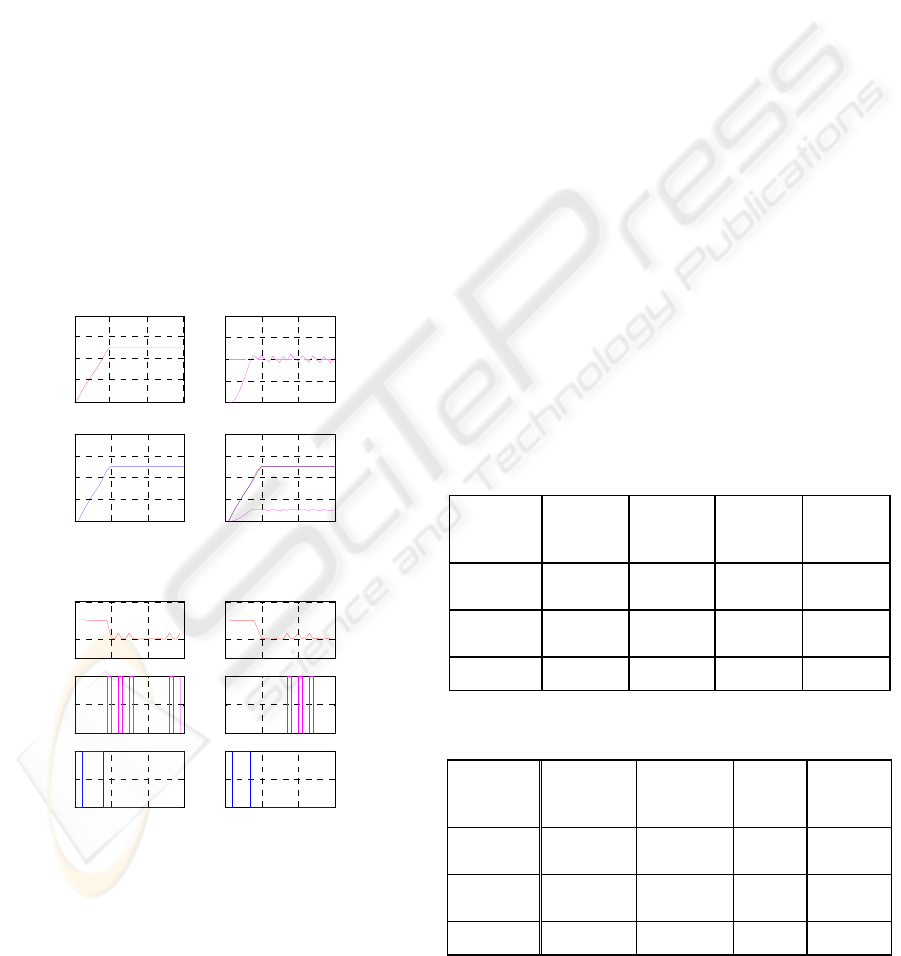
Let us consider now the following specification:
starting from zero levels (the three tanks being
completely empty), the objective of the control
strategy is to reach the liquid levels
m 5.0
1
=
h ,
and . The MPC technique for
a SPMLD model has been implemented in
simulation to reach the level specification with
. The results are presented on Figure 5 for the
tanks levels and on Figure 6 for the control signals.
m 5.0
2
=h m 1.0
3
=h
2=N
10 20 30
0
0.2
0.4
0.6
0 10 20 30
0
0.2
0.4
0.6
0.8
0 10 20 30
0
0.05
0.1
0.15
0.2
0 10 20 30
0
0.2
0.4
0.6
0.8
Level of the frist tank
Level of the third tank
Level of the second tank
The level of three tanks
Sampling instants
Sampling instants
Figure 5: Water levels in the three tanks
0 10 20 30
0
2
x 10
-4
The flow (m
3
/5)
0 10 20 30
0
2
x 10
-4
0 10 20 30
0
0.5
1
The valve position
1 (open) - 0 (close)
0 10 20 30
0
0.5
1
0 10 20 30
0
0.5
1
0 10 20 30
0
0.5
1
Input Q1
Input Q2
V1 V2
V13
V23
Sampling instants
Sampling instants
Figure 6: Controlled variables
The level of the third tank oscillates around 0.1 as
does not correspond to an equilibrium
point. Consequently, the system opens and closes the
two valves
1
V and
2
V to maintain the level in the
third tank around the desired level of 0.1m.
1.0
3
=h
5.3 Comparison of the approaches
As a comparison purpose between the SPMLD
model, the classical MLD model and the classical
PWA model strategies, the same previous level
specification has been considered with
. The
MLD model described in (Bemporad et al., 1999)
has been used for the three tanks modeled by (20);
this MLD model transfers to a PWA model with
2=N
128
=
s subsystems (with 28 empty regions). The
classical PWA model has not been developed as it
needs 100 sub-models and is in fact not required to
compare complexity. For that comparison, looking
at the number of QPs that have to be solved during
optimization is sufficient.
Table 1 illustrates for
the total time
required to reach the specification level, the total
number of QPs solved, and the maximum time and
maximum QPs to find the optimized solution at each
iteration. It can be seen that the difference between
the SPMLD technique and the other classical
techniques is quite large, the SPMLD model
allowing real time implementation and avoiding
exponential explosion of the algorithm (the sampling
time of the three tanks benchmark is 10 s.). All data
given above were obtained using the MIQP Matlab
code (Bemporad and Mignone, 2000), on a 1.8 MHz
PC with 256 Mo of ram. Same comparisons are
presented with
2=N
3
=
N in table 2.
Table 1: Comparison of performances obtained with the
SPMLD model, the classical MLD model and the classical
PWA model for 2
=
N .
Approach
No of
QPs
solved
Max.
No. QPs
/ step
Total
time
Max.
time /
step
Classical
PWA
8 800 1 600 * *
Classical
MLD
11 130 2 089 822.97 s 138.97 s
SPMLD 832 218 15.28 s 3.90 s
Table 2: Comparison of performances obtained with the
SPMLD, MLD and PWA models for
3=N
Approach
No of QPs
solved
Max. No.
QPs / step
Total
time
Max.
time /
step
Classical
PWA
880 000 160 000 * *
Classical
MLD
25 606 6 867
5243.6
s
1 147.80
s
SPMLD 3 738 1 054 137.54 s 37.65 s
This table shows that no real time implementation is
possible with
3
=
N for the SPMLD form, although
the maximum time per iteration is much smaller in
ICINCO 2004 - SIGNAL PROCESSING, SYSTEMS MODELING AND CONTROL
84

this case. But it must be noticed that the results in
table 1 and 2 for the SPMLD model are achieved
without applying techniques described in section
4.4. For example using a prediction horizon
3
=
N
and a control horizon
1
=
u
N leads to the following
results enabling real time implementation
No QPs solved = 1224, Max. No QPs/step = 326
Total optimization time = 29.24 s., Max. time/step = 7.92 s.
The technique of MPC for SPMLD systems has
been examined also with a simple automata, where
automata of Figure 7 have been added to
1
V and
2
V
valves of the three tanks benchmark. We assumed
for a simplification purpose that
03
0=
δ
i.e. the
level in the third tank is always behind the h
v
level.
V
1
open
Wait
V
2
open
a b
close
close
close a
b
Figure 7: added Automata to the three tanks benchmark.
The automata of Figure 7 can be presented as follows
closeWait
bVbwaitV
aVawaitV
openopen
openopen
=
=
=
)&()&(
)&()&(
22
11
(23)
The SPMLD technique succeeds to reduce the total
optimization time to arrive to the specifications,
from 5691.4 s for the classical MLD technique to a
173.5 s, solving 3990 QPs instead of 60468 QPs
where for each sequence I,
variables as well as
the logical control variables that control the
automata are known.
δ
6 CONCLUSION
This paper presents the SPMLD formalism. It is
developed by partitioning the feasible region
according to the auxiliary binary elements
1
of the
MLD model that depends on the state variables. A
reformulation of the MPC strategy for this
formalism has been presented. It is shown that the
SPMLD model successfully improves the
computational problem of the mixed Logical
Dynamical (MLD) model and Piecewise Affine
(PWA) model. Moreover, the partition into several
sub-regions enables to define particular weighting
factors according to the priority of each region.
Future work may consider examining
variables
that depends on the control inputs, by partitioning
the feasible region according to those variables also
instead of leaving them free included in the
optimization vector.
δ
δ
REFERENCES
Bemporad, A., 2003. “A Recursive Algorithm for
Converting Mixed Logical Dynamical Systems into an
Equivalent Piecewise Affine Form”, IEEE Trans.
Autom. Contr.
Bemporad, A., Ferrari-Trecate G., and Morari M., 2000.
Observability and controllability of piecewise affine
and hybrid systems. IEEE Trans. Automatic Control,
45(10):1864–1876.
Bemporad, A., and Mignone, D., 2000.: Miqp.m: A
Matlab function for solving mixed integer quadratic
programs. Technical Report.
Bemporad, A., Mignone, D. and Morari, M., 1999.
Moving horizon estimation for hybrid systems and
fault detection. In Proceedings of the American
Control Conference, San Diego.
Bemporad, A. and Morari, M., march 1999. Control of
systems integrating logical, dynamics, and constraints.
Automatica, 35(3):407-427.
Branicky, M.S., Borkar, V.S. and Mitter, S.K., January
1998. A unified framework for hybrid control: model
and optimal control theory. IEEE Transaction. on
Automatic. Control, 43(1): 31-45.
Dolanc, G., Juricic D., Rakar A., Petrovcic J. and Vrancic,
D., 1998. Three-tank Benchmark Test. Technical
Report Copernicus Project Report CT94-02337.
Dumur, D. and Boucher, P.,1998. A Review Introduction
to Linear GPC and Applications. Journal A, 39(4),
pp. 21-35.
Fletcher, R. and Leyffer, S., 1995. Numerical experience
with lower bounds for MIQP branch and bound.
Technical report, Dept. of Mathematics, University of
Dundee, Scotland.
Kerrigan, E., 2000. Robust Constraint Satisfaction:
Invariant sets and predictive control. PhD thesis
University of Cambridge.
Pena, M.., Camacho, E. F. and Pinon, S., 2003. Hybrid
systems for solving model predictive control of
piecewise affine system. IFAC conference, Hybrid
system analysis and design Saint Malo, France.
Sontag, E.D., April 1981: Nonlinear regulation: the
piecewise linear approach. IEEE Transaction. on
Automatic. Control, 26(2):346-358.
Torrisi, F., Bemporad, A. and Mignone, D., 2000. Hysdel
– a tool for generating hybrid models. Technical
report, AUT00-03, Automatic control laboratory, ETH
Zuerich.
MODEL PREDICTIVE CONTROL FOR HYBRID SYSTEMS UNDER A STATE PARTITION BASED MLD
APPROACH (SPMLD)
85
