PARTIAL VIEWS MATCHING USING A METHOD BASED ON

PRINCIPAL COMPONENTS

Santiago Salamanca Mi

Universidad de Extremadura (UEX)

Escuela de Ingenir

ıas Industriales. Badajoz. Spain

Carlos Cerrada Somolinos

Universidad Nacional de Educaci

on a Distancia (UNED)

Escuela T

ecnica Superior de Ingenier

ıa Industrial. Madrid. Spain

Antonio Ad

an Oliver

Universidad de Castilla la Mancha (UCLM)

Escuela Superior de Ingenier

ıa Inform

atica. Ciudad Real. Spain

Miguel Ad

an Oliver

Universidad de Castilla la Mancha (UCLM)

Escuela Universitaria de Ingenier

ıa T

ecnica Agr

ıcola. Ciudad Real. Spain

Keywords:

Matching, recognition, unstructured range data, 3D computer vision.

Abstract:

This paper presents a method to estimate the pose (position and orientation) associated to the range data of an

object partial view with respect to the complete object reference system. A database storing the principal com-

ponents of the different partial views of an object, which are generated virtually, is created in advance in order

to make a comparison between the values computed in a real view and the stored values. It allows obtaining

a ﬁrst approximation to the searched pose transformation, which will be afterwards reﬁned by applying the

Iterative Closest Point (ICP) algorithm.

The proposed method obtains very good pose estimations achieving very low failure rate, even in the case of

the existence of occlusions. The paper describes the method and demonstrates these conclusions by presenting

a set of experimental results obtained with real range data.

1 INTRODUCTION

Relative pose of the partial view of an object in a

scene with respect to the reference system attached to

the object can be determined by using matching tech-

niques. This work is concerned with the problem of

matching 3D range data of a partial view over the 3D

data of the complete object. Resolution of this prob-

lem is of utmost practical interest because it can be

used in applications like industrial robotics, mobile

robots navigation, visual inspection, etc.

A standard way of dealing with this problem is to

generating a model from the data, which allows ex-

tracting and representing some information associated

to the source data. There are two basic classes of rep-

resentation (Mamic and Bennamoun, 2002): object

based representations and view based representations.

In the ﬁrst class, models are created by extracting

representative features of the objects. This type can be

divided into four major categories: boundaries repre-

sentations, generalized cylinders, surface representa-

tions and volumetric representations, being the third

one the mostly used. In this case, a surface is ﬁtted

from the range data and then certain features are ex-

tracted from the ﬁtted surface. Spherical representa-

tions belong to this category, being the Simplex An-

gle Image (SAI) representation (Higuchi et al., 1994;

Hebert et al., 1995; Ad

an et al., 2001b; Ad

an et al.,

2001a) an important example of this type of surface

representation. In general terms, object based repre-

sentations are not the most suitable ones for applica-

tion in partial views matching.

Concerning to the view based representations they

try to generate the model as a function of the di-

verse appearances of the object from different points

of view. There exist a lot of techniques that belong to

Salamanca Miño S., Cerrada Somolinos C., Adán Oliver A. and Adán Oliver M. (2004).

PARTIAL VIEWS MATCHING USING A METHOD BASED ON PRINCIPAL COMPONENTS.

In Proceedings of the First International Conference on Informatics in Control, Automation and Robotics, pages 3-10

DOI: 10.5220/0001137200030010

 SciTePress

this class (Mamic and Bennamoun, 2002). Let us re-

mark the methods based in principal components (PC)

(Campbell and Flynn, 1999; Skocaj and Leonardis,

2001), which use them in the matching process as dis-

criminant parameters to reduce the initial range im-

ages database of an object generated from all possible

viewpoints.

The method presented in this paper can be classi-

ﬁed halfway of the two classes because the appear-

ance of the object from all the possible points of

view are not stored and managed. Instead of that,

only some features of each view are stored and han-

dled. More speciﬁcally, just three critical distances

are established from each point of view. These dis-

tances are determined by means of the principal com-

ponents computation. A ﬁrst approach to the transfor-

mation matrix between the partial view and the com-

plete object can be obtained from this computation.

The deﬁnitive transformation is ﬁnally achieved by

applying a particular version of the Iterative Closest

Point (ICP) algorithm (Besl and McKay, 1992) to the

gross transformation obtained in the previous stage.

A comparative study of different variants of the ICP

algorithm can be seen in (Rusinkiewicz and Levoy,

2001).

The paper is organized as follows. A general de-

scription of the overall method is exposed in the next

section. The method developed to obtain the database

with the principal components from all the possible

viewpoints are described is section 3. Section 4 is de-

voted to present the matching algorithm built on top

of the principal components database. A set of exper-

imental results is shown in section 5 and conclusions

are stated in section 6.

2 OVERALL DESCRIPTION OF

THE METHOD

As it has been mentioned, the ﬁrst stage of the pro-

posed method is based on the computation of the prin-

cipal components from the range data corresponding

to a partial view. Let us call X to this partial view.

Principal components are deﬁned as the set of eigen-

values and eigenvectors {(λ

, ˜e

) |i = 1, . . . , m} of

the Q covariance matrix:

Q = X

(1)

where X

represents the range data translated with

respect to the geometric center.

In the particular case we are considering, X

is a

matrix of dimension n × 3 and there are three eigen-

vectors that point to the three existing principal direc-

tions. The ﬁrst eigenvector points to the spatial direc-

tion where the data variance is maximum. From a ge-

ometrical point of view, and assuming that the range

data is homogeneously distributed, it means that the

distance between the most extreme points projected

over the ﬁrst direction is the maximum among all pos-

sible X

couple of points. The second vector points

to another direction, normal to the previous one, in

which the variance is maximum for all the possible

normal directions. It means again that the distance

between the most extreme points projected over the

second direction is the maximum among all the pos-

sible directions normal to the ﬁrst vector. The third

vector makes a right-handed reference system with

the two others. The eigenvalues represent a quantita-

tive measurement of the maximum distances in each

respective direction.

From the point of view of its application to the

matching problem it is important to remark ﬁrstly that

the eigenvalues are invariant to rotations and trans-

lations and the eigenvectors invariant to translations,

and secondly that the frame formed by the eigenvec-

tors represents a reference system ﬁxed to the own

range data. The ﬁrst remark can be helpful in the

process of determining which portion of the complete

object is being sensed in a given partial view, i.e. the

recognition process. The second one gives an initial

estimation of the searched transformation matrix that

matches the partial view with the complete object in

the right pose. In fact, it is only valid to estimate the

rotation matrix because the origins of the reference

systems do not coincide.

To implement the recognition process it is neces-

sary to evaluate, in a previous stage, all the possible

partial views that can be generated for a given com-

plete object. We propose a method that considers a

discretized space of the viewpoints around the object.

Then a Virtual Partial View (VPV) is generated for

all the discretized viewpoints using a z-buffer based

technique. Principal components of each one of these

VPV are then computed and stored, such that they can

be used in the recognition process.

Initial information of the possible candidate zones

to matching a sample partial view to the complete ob-

ject can be extracted by comparing the eigenvalues of

the sample with the stored values. Nevertheless, this

is only global information and it only concerns to ori-

entation estimation. A second process must be imple-

mented in order to obtain a ﬁne estimate of the ﬁnal

transformation matrix. We use the ICP algorithm ap-

plied to the set of candidates extracted in the previous

process. The transformation matrix estimated from

the eigenvectors is used as the initial approximation

required by the ICP algorithm. The ﬁnal matching

zone is selected as the one that minimizes the ICP er-

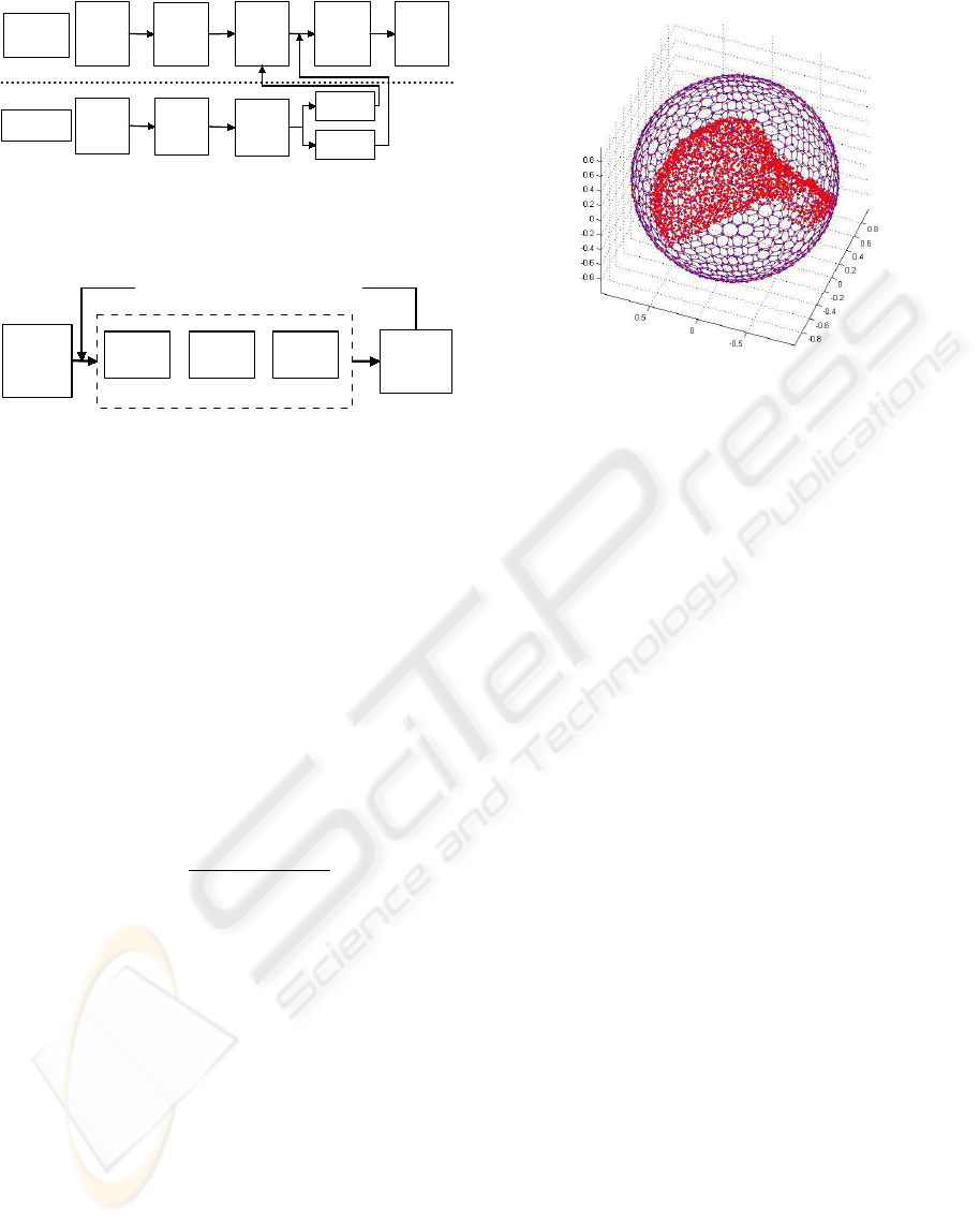
ror. Figure 1 shows a schematic block diagram of the

entire developed method. More implementation de-

tails are explained in next sections.

ICINCO 2004 - ROBOTICS AND AUTOMATION

Transformation

computation

process

Range data of

the sample

partial view PV

PV principal

components

computation

Eigenvalues

comparison

(View Point

estimation)

Initial

Transformation

matrix

estimation

ICP algorithm

application.

Final

transformation

matrix

computation

Model

generation process

(off-line)

Range data of

the complete

object

Virtual Partial

Views ( VPV)

computation

Principal

Components

of the VPV

computation

Eigenvalues

storage

Eigenvectors

storage

Figure 1: Block Diagram of the proposed method to ﬁnd

the best match of a given range data partial view with the

complete object.

Range data of

the complete

object

(input data)

Principal

Components

of the VPV

computation

Repeat for all the view points around the object

Multipixel

image

generation

z-buffer

algorithm

application

Data filtering

Virtual Partial View (VPV) computation

Figure 2: Block diagram of the process followed to generate

the principal components database.

3 PRINCIPAL COMPONENTS

DATABASE GENERATE

A database storing the principal components of all the

possible partial views that can be generated from the

range data of a given complete object must be com-

puted in an off-line previous stage. Figure 2 shows

the steps followed in this process.

Range data of the complete object is ﬁrstly trans-

lated to its geometric center and then normalized to

the unit value. Therefore, we will start to work with

the following normalized range data:

M − c

max (kM − ck)

(2)

where M is the range data of the complete object, c

is the geometric center, max is the maximum function

and || · || is the Euclidean distance. At this point, as

can be observed in Figure 2, the most important step

of the method is the computation of the virtual partial

views (VPV) described in the next subsection.

3.1 Virtual Partial Views

Computation

A VPV can be deﬁned as a subset of range data points

O ⊂ M

virtually generated from a speciﬁc view-

point VP, and that can be approximated to the real par-

tial view obtained with a range sensor from the same

VP.

Notice that in this deﬁnition it is necessary to con-

sider, apart from the object range data itself, the view-

point from which to look at the object. In order to

Figure 3: Visual space discretization around the complete

object range data. Each sphere node constitutes a different

viewpoint from which a VPV is estimated.

take into account all the possible viewpoints, a dis-

cretization of the visual space around the object must

be considered. A tessellated sphere circumscribed to

the object is used for that and each node of the sphere

can be considered as a different and homogeneously

distributed viewpoint from where to generate a VPV

(see Figure 3).

For a speciﬁc VP its corresponding virtual partial

view is obtained by applying the z-buffer algorithm.

This algorithm is widely used in 3D computer graph-

ics applications and it allows deﬁning those mesh

patches that can be viewed from a given viewpoint.

Speciﬁcally, only the facets with the highest value of

the z component will be visible, corresponding the Z-

axis with the viewing direction.

This method is designed to apply when there is

information about the surfaces to visualize, but not

when just the rough 3D data points are available.

Some kind of data conversion must be done previous

to use the algorithm as it is. We have performed this

conversion by generating the named multipixel matrix

of the range data. This matrix can be obtained as fol-

lows. First a data projection over a plane normal to

the viewing direction is performed:

= UM

(3)

where U is the matrix representing such projection.

This transformation involves a change from the orig-

inal reference system S = {O, X, Y, Z} to the new

one S

= {OX

} where the Z’ component, de-

noted as z’, directly represents the depth value. From

these new data an image can be obtained by discretiz-

ing the X’Y’ plane in as many pixels as required, and

by assigning the z’ coordinate of each point as the im-

age value. Notice that in this process several points

can be associated to the same pixel if they have the

PARTIAL VIEWS MATCHING USING A METHOD BASED ON PRINCIPAL COMPONENTS

Projected

2D points

Depth

3D points with the

same 2D projection

Figure 4: Multipixel matrix representation

Figure 5: Visualization of each one of the planes of the mul-

tipixel matrix as a compacted intensity image

same (x’,y’) coordinate values. To avoid depth infor-

mation loss in these cases, the image values are stored

in a three dimensional matrix. For that reason the cre-

ated structure is denoted as multipixel matrix.

Figure 4 shows a typical scheme of this matrix. On

the other hand, ﬁgure 5 shows as a grey-scaled image

and in a compacted manner all the two-dimensional

matrices that conform this structure. Pixels next to

white color represent higher z’ values. Figure 6 shows

an image obtained by selecting for each pixel the

maximum of its associated z’ values. If the data points

corresponding to these selected z’ values are denoted

as O

⊂ M

, then the VPV can be obtained by ap-

plying the inverse of the U transformation deﬁned in

equation (3), i.e.:

O = U

−1

(4)

The set of range data points corresponding to a

VPV obtained after the application of the described

process to a sample case can be seen in the ﬁgure 7 (a)

and (b). It can be observed that results are generally

acceptable but some spurious data appear. These val-

ues were already noticeable from ﬁgure 6 where they

look like a salt-pepper noise effect. Due to this fact,

a median ﬁlter (see ﬁgure 8) is applied to the image

before evaluating the equation (4), in order to obtain

the deﬁnitive range data points of the searched VPV

(ﬁgure 9).

Figure 6: Intensity image associated to the maximum value

of z

at each pixel.

(b)

Spurious data

(a)

Figure 7: Range data points corresponding to a Virtual Par-

tial View. They are shown from two different points of view

to improve their visualization. In (b) the existence of spuri-

ous data are more evident.

Figure 8: Image obtained after applying a median ﬁlter to

the image shown in ﬁgure 6

ICINCO 2004 - ROBOTICS AND AUTOMATION

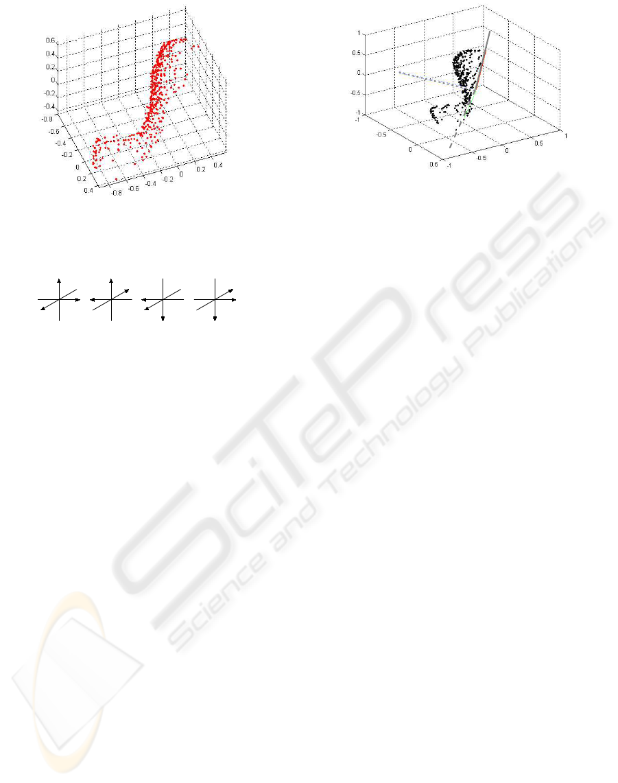
Figure 9: Deﬁnitive range data of a VPV. It can be observed,

comparing with the ﬁgure 7(b), that the noise has been re-

moved

X

Y

Z

X

Y

Z

X

Y

Z

Y

Z

X

Figure 10: Four ambiguous frames for direction combina-

tions

3.2 Principal Components of VPV

Computation

Once the range data points of a VPV have been de-

termined the associated principal components can be

computed from them. They will be the eigenvectors

and the eigenvalues of the covariance matrix at (1),

where X

is now O.

Due to the fact that the eigenvectors only provide

information about the line vectors but not about their

directions, some uncertainties can appear in the ul-

terior matching process. For example, using right

handed coordinate systems like in ﬁgure 10, if no di-

rection is ﬁxed in advance there are four ambiguous

possibilities for frame orientation. It can be also seen

in the ﬁgure 10 that when one of the line directions is

ﬁxed only two possibilities appear, being related one

to the other by a rotation of π radians around the ﬁxed

axis. For that reason, before storing the VPV eigen-

vectors, following steps are applied:

1. Verify if the third eigenvector forms an angle

smaller than π/2 with the viewing direction. If not,

we take the opposite direction for this eigenvector.

2. The ﬁrst eigenvector direction is taken to build to-

gether with the two others a right-handed frame.

After these steps, principal components of the VPV

are stored in the database for posterior use in the

matching process. Figure 11 shows the deﬁnitive

principal components of a given VPV.

Figure 11: Deﬁnitive eigenvectors computed from the range

data of a VPV. The ﬁrst one is represented in red, second in

green and the third in blue.

4 MATCHING PROCESS

The developed matching process is divided in four

stages (see ﬁgure 1):

1. Principal components computation of the acquired

partial view.

2. eigenvalues comparison and initial candidates

zones selection.

3. Initial transformation estimation by using the

eigenvectors.

4. ICP algorithm application to determine the ﬁnal

transformation.

The method developed to carry out the three ﬁrst

stages is described in the next subsection. Then we

will explain how the ICP algorithm is applied to ob-

tain the ﬁnal result.

4.1 Initial Transformation Matrix

Computation

The ﬁrst thing to do is to compute the eigenvectors

and eigenvalues of the acquired range partial view.

To maintain equivalent initial conditions than in the

VPV computation we must apply the same steps ap-

plied to the complete object range data: normalization

with respect to the geometric center of the complete

object, M; multipixel matrix generation; z-buffer al-

gorithm application and, ﬁnally, data ﬁltering. In this

case the main objective is to try the handled data being

the most similar possible to those used in the principal

component computation of the VPV.

After that, the principal components are computed

and the deﬁnitive vector directions are established fol-

lowing the steps described in subsection 3.2. Then the

eigenvalues of the acquired view are compared with

the eigenvalues of all the stored VPV by evaluating

the following error measurement:

PARTIAL VIEWS MATCHING USING A METHOD BASED ON PRINCIPAL COMPONENTS

(a) (b) (c)

Figure 12: Results of the comparing eigenvectors algo-

rithm. (a) Visualization of the acquired range data partial

view. (b) Five selected candidate viewpoints from e

error

computation. (c) Rotated data results for the ﬁrst candidate

= ||Λ

− Λ

|| (5)

where Λ

= {λ

, λ

} is the vector formed by the

eigenvalues of a VPV, Λ

= {λ

, λ

} is the vector

formed by the eigenvalues of the real partial view and

|| · || is the Euclidean distance.

Notice that a given VPV can achieve the minimum

value of e

and not being the best candidate. This

is because the feature we are using is a global one.

For that reason we take a set of selected candidates to

compute the possible initial transformation. Speciﬁ-

cally, we are selecting the ﬁve VPV candidates with

less error.

These initial transformations do not give the exact

required rotation to coupling the eigenvector because

the original data are not normalized with respect the

same geometric center. Mathematically, what we are

computing is the rotation matrix R such that applied

to the eigenvectors of the real partial view, E

, gives a

set of eigenvectors coincident with the VPV ones, E

Because both E

and E

represent orthonormal ma-

trices, the searched rotation matrix can be computed

from the next expression:

R = E

)

−1

= E

)

(6)

Because of the ambiguity of the two possible di-

rections existing in the eigenvectors deﬁnition, the ﬁ-

nal matrix can be the directly obtained in (6) or an-

other one obtained after rotating an angle of π radians

around the third eigenvector.

Figure 12 shows the results of the comparing eigen-

vectors algorithm. In (a) the real partial view is

shown. The ﬁve selected candidates with less e

er-

ror values are remarked over the sphere in part (b).

An arrow indicates the ﬁrst candidate, i.e. the corre-

sponding to the minimum e

value. The approximate

R matrix obtained as a result of equation (6) evalua-

tion can be observed in (c). In this case the result cor-

responds to the VPV associated to the ﬁrst candidate

viewpoint. Deﬁnitive matrix will be obtained after a

reﬁnement process by means of the ICP algorithm ap-

plication.

Summarizing, the resulting product of this phase is

a transformation matrix T whose sub matrix R is ob-

tained from equation (6) and whose translation vector

is t = [0, 0, 0]

4.2 ICP Algorithm Application

The Iterative Closest Point (ICP) (Besl and McKay,

1992) is an algorithm that minimizes the medium

quadratic error

e(k) =

||P − P

(7)

among the n data points of an unknown object P’,

called scene data, and the corresponding data of the

database object P, called model data. In our particu-

lar case, the scene data are the range data of the real

partial view, X

, normalized and transformed by the

T matrix, and the model data are the subset of points

of the complete object M

that are the nearest to each

of the scene points. The latest will change at each it-

eration step.

Once the model data subset in a given iteration step

k are established, and assuming that the error e(k) is

still bigger than the ﬁnishing error, it is necessary to

determine the transformation matrix that makes min-

imum the error e(k). Solution for the translation part,

the t vector, is obtained from the expression (Forsyth

and Ponce, 2002):

t =

i=1

−

i=1

(8)

where r

and r

are the coordinates of the model data

points and scene data points respectively.

With respect to the rotation part, the rotation matrix

R that minimizes the error, we have used the Horn

approximation (Horn, 1988), in which R is formed by

the eigenvectors of the matrix M deﬁned as:

M = P (P

)

(9)

This approximation gives a closed-form solution

for that computation, which accelerates signiﬁcantly

the ICP algorithm.

The algorithm just described is applied to the ﬁve

candidates selected in the previous phase. The chosen

ﬁnal transformation matrix will be that one for which

the ﬁnishing ICP error given by expression (7) is the

smaller one.

Figure 13 shows the results for the same data points

of ﬁgure 11 after application of the ICP algorithm.

Partial view after applying the ﬁnal transformation

matrix matched over the object and the complete ob-

ject range data are plotted together. Plots from two

different points of view are shown to improve the vi-

sualization of the obtained results.

ICINCO 2004 - ROBOTICS AND AUTOMATION

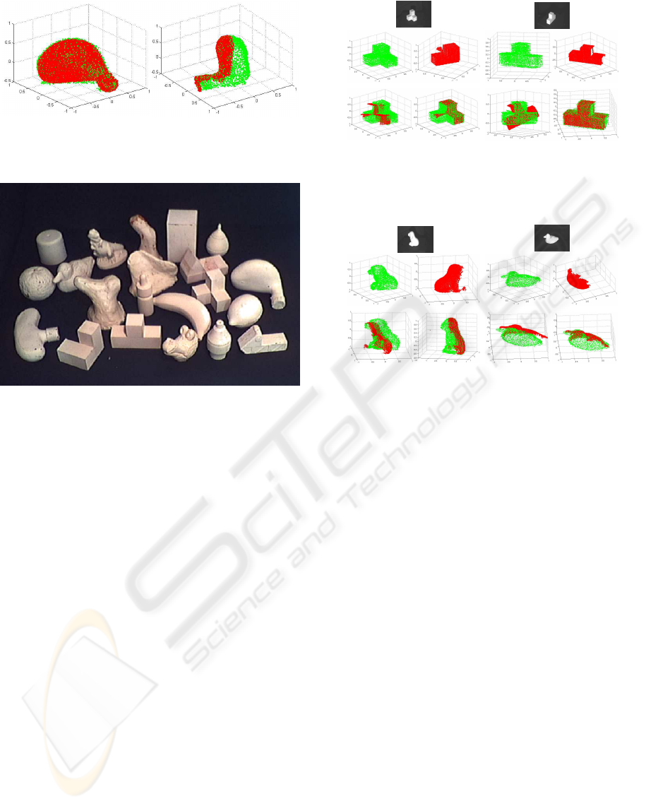
Figure 13: Final results of the overall matching algorithm

visualized from two different points of view

Figure 14: Set of objects used to test the presented algo-

rithm

5 EXPERIMENTAL RESULT

The algorithm proposed in the present work has been

tested over a set of 21 objects. Range data of these ob-

jects have been acquired by means of a GRF-2 range

sensor which provides an average resolution of ap-

proximately 1 mm. Real size of the used objects goes

from 5 to 10 cm. height and there are both polyhedral

shaped and free form objects (see ﬁgure 14).

We have used a sphere with 1280 nodes to com-

pute the principal components for the complete ob-

ject. Some tests have been made with a mesh of 5120

nodes, but the associated increment of the computa-

tion time does not bring as a counterpart any improve-

ment in the obtained matching results.

With respect to the multipixel matrix, sizes around

22x22 pixels have empirically given good results. The

matrix size can be critical in the method functionality

because high value implies poor VPV generation, and

low value involves a reduction in the number of range

data points that conform the VPV, making unaccept-

able the principal components computation.

Once the principal components database was gen-

erated for all the considered objects we have checked

the matching algorithm. Three partial views have

been tested for each object, making a total of 63 stud-

ied cases. The success rate has been the 90,67%, what

(a) (b)

(c) (d)

Object 1

(a) (b)

(c) (d)

Object 2

Figure 15: Some results over polyhedral objects of the pro-

posed method

(a) (b)

(c) (d)

Object 3

(a) (b)

(c) (d)

Objeto 4

Figure 16: Some results over free form objects of the pro-

posed method

demonstrates the validity of the method.

The average computation time invested by the algo-

rithm has been 75 seconds, programmed over a Pen-

tium 4 at 2.4 GHz. computer under Matlab environ-

ment. The time for the phase of eigenvalues com-

parison and better candidates’ selection is very small,

around 1 sec. The remaining time is consumed in the

computation of the principal components of the real

partial view and, mainly, in the application of the ICP

algorithm to the ﬁve candidates: ﬁve times for the di-

rect computation of the R matrix from equation (6),

and another ﬁve times due to the direction ambigu-

ity existing in the eigenvectors deﬁnition described in

subsection 3.2.

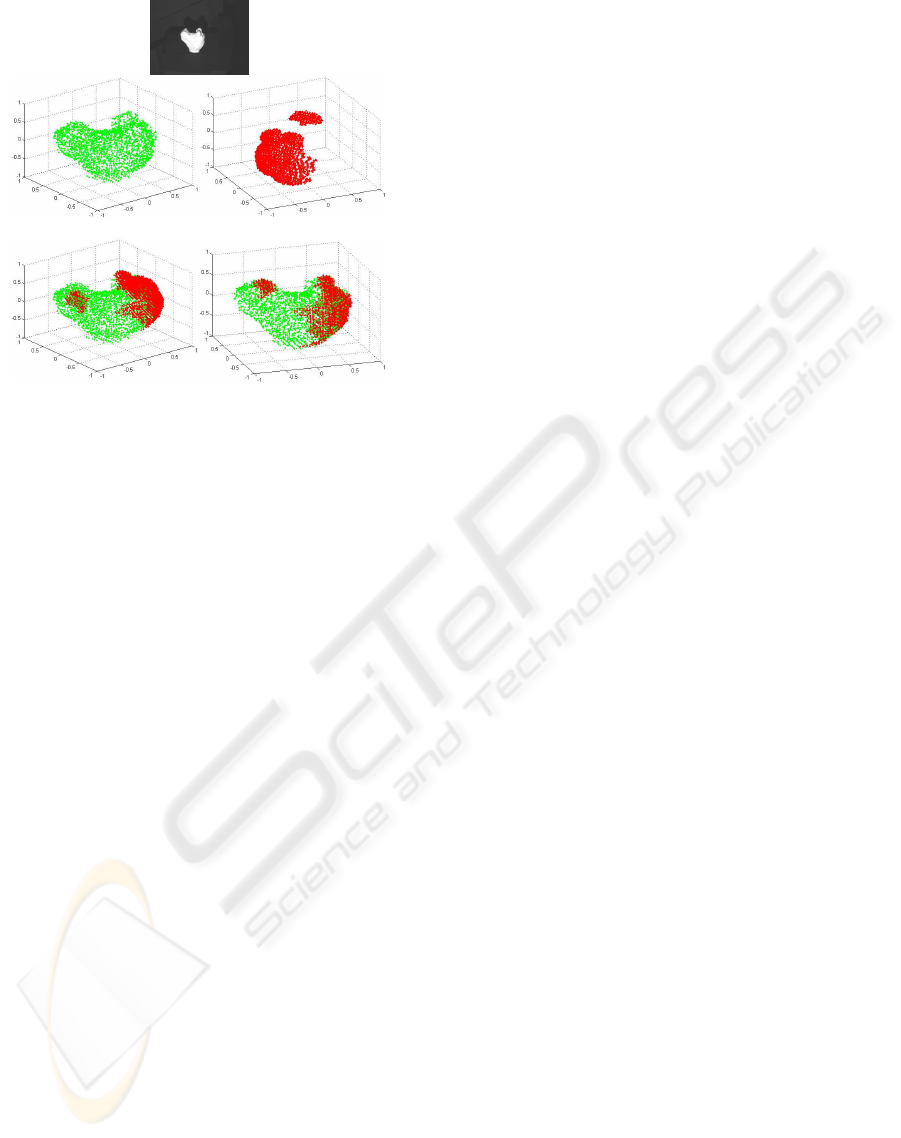
Figures 15 and 16 show the results obtained with

several polyhedral and free-form objects respectively.

Apart from the intensity image of the object, sub-

plot (a) presents the range data of the complete ob-

ject, subplot (b) shows the partial view set of points,

subplot (c) shows the data transformed after eigen-

values comparison, and subplot (d) contains the ﬁnal

results after ICP algorithm application. Some plots

have been rotated to enhance data visualization.

Finally it is important to remark that the devel-

oped algorithm can handle partial views with auto-

occlusions. Figure 17 shows an example of this case.

PARTIAL VIEWS MATCHING USING A METHOD BASED ON PRINCIPAL COMPONENTS

(a) (b)

(c) (d)

Object 4

Figure 17: Results of the method in a free form object with

existence of auto occlusions

6 CONCLUSIONS

A method to ﬁnd the best matching of a range data

partial view with the complete object range data has

been presented in this work. The method takes ad-

vantage of the principal components concept. The

eigenvalues comparison allows determining the most

probable matching zones among the partial view and

the complete object. The corresponding eigenvectors

are used to compute an initial transformation matrix.

Applying the ICP algorithm reﬁnes this one and the

deﬁnitive transformation is obtained.

For the comparison purposes a database of prin-

cipal components must be generated in advance. A

procedure has been designed and described to virtu-

ally generate all the possible partial views of a given

complete object and then to compute the associated

principal components. The procedure is based on the

z-buffer algorithm.

The method has been tested over a database con-

taining 21 objects, both polyhedral and free form, in a

63 case study (three different views for each object).

The success rate has been the 90,67%. The method

has proven its robustness to auto-occlusions. Some

improvements can still to be made in a future concern-

ing to the candidate selection step. Several candidates

appear at the same zone and they could be grouped

into the same one for the following step of ICP appli-

cation.

Finally it is important to remark that the pre-

sented method has very good performance in the

shown matching problem but it can also be applied

in recognition applications with similar expected per-

formance.

ACKNOWLEDGEMENTS

This work has been developed under support of the

Spanish Government through the CICYT DPI2002-

03999-C02-02 contract.

REFERENCES

an, A., Cerrada, C., and Feliu, V. (2001a). Automatic

pose determination of 3D shapes based on modeling

wave sets: a new data structure for object modeling.

Image and Vision Computing, 19(12):867–890.

an, A., Cerrada, C., and Feliu, V. (2001b). Global shape

invariants: a solution for 3D free-form object discrim-

ination/identiﬁcation problem. Pattern Recognition,

34(7):1331–1348.

Besl, P. and McKay, N. (1992). A method for registration

of 3-D shapes. IEEE Transactions on Pattern Analysis

and Machine Intelligence, 14(2):239–256.

Campbell, R. J. and Flynn, P. J. (1999). Eigenshapes for 3D

object recognition in range data. In Proc. of the IEEE

Conference on Computer Vision and Pattern Recogni-

tion, volume 2, pages 2505–2510.

Forsyth, D. A. and Ponce, J. (2002). Computer Vision: A

Modern Approach. Prentice Hall.

Hebert, M., Ikeuchi, K., and Delingette, H. (1995). A

spherical representation for recognition of free-form

surfaces. IEEE Transactions on Pattern Analysis and

Machine Intelligence, 17(7):681–690.

Higuchi, K., Hebert, M., and Ikeuchi, K. (1994). Merg-

ing multiple views using a spherical representation. In

IEEE CAD-Based Vision Workshop, pages 124–131.

Horn, B. K. (1988). Closed form solutions of absolute ori-

entation using orthonormal matrices. Journal of the

Optical Society A, 5(7):1127–1135.

Mamic, G. and Bennamoun, M. (2002). Representation and

recognition of 3D free-form objects. Digital Signal

Processing, 12(1):47–76.

Rusinkiewicz, S. and Levoy, M. (2001). Efﬁcient variants

of the ICP algorithm. In Proceeding of the Third Inter-

national Conference on 3D Digital Imaging and Mod-

eling (3DIM01), pages 145–152, Quebec, Canada.

Skocaj, D. and Leonardis, A. (2001). Robust recognition

and pose determination of 3-D objects using range im-

age in eigenspace approach. In Proc. of 3DIM’01,

pages 171–178.

ICINCO 2004 - ROBOTICS AND AUTOMATION