A NOVEL REPETITIVE CONTROL ALGORITHM COMBINING ILC
AND DEAD-BEAT CONTROL
C. Freeman, P. Lewin and E. Rogers
School of Electronics and Computer Science, University of Southampton
Highfield, SO17 1BJ, United Kingdom
J. Hätönen, T. Harte and D.H. Owens
Department of Automatic Control and Systems Engineering, University of Sheffield
Mappin Street, Sheffield S1 3JD, United Kingdom
Keywords:
Iterative Learning Control, Repetitive Control, Dead-beat control
Abstract:
In this paper it is explored whether or not a well-known adjoint Iterative Learning Control (ILC) algorithm
can be applied to Repetitive Control (RC) problems. It is found that due to the lack of resetting in Repetitive
Control, and the non-causal nature of the adjoint algorithm, the implementation requires a truncation procedure
that can lead to instability. In order to avoid the truncation procedure, as a novel idea it is proposed that dead-
beat control can used to shorten the impulse response of the plant to be so short that the need for truncation is
removed. Therefore, convergence is guaranteed, if the adjoint algorithm is applied to the closed-loop plant with
a dead-beat controller. The proposed algorithm is validated using real-time experiments on a non-minimum
phase spring-mass-damper system. The experimental results show fast convergence to near perfect tracking,
demonstrating the applicability of the proposed algorithm to industrial RC problems.
1 INTRODUCTION
Many signals in engineering are periodic, or at least
they can be accurately approximated by a periodic
signal over a large time interval. This is true, for ex-
ample, of most signals associated with engines, elec-
trical motors and generators, converters, or machines
performing a task over and over again. Hence it is an
important control problem to try to track a periodic
signal with the output of the plant or try to reject a
periodic disturbance acting on a control system.
In order to solve this problem, a relatively new re-
search area called Repetitive Control has emerged in
the control community. The idea is to use information
from previous periods to modify the control signal so
that the overall system would ‘learn’ to track perfectly
a given T -periodic reference signal. The first paper
that uses this ideology seems to be (Inouye et al.,
1981), where the authors use repetitive control to ob-
tain a desired proton acceleration pattern in a proton
synchrotron magnetic power supply. Since then repet-
itive control has found its way to several practical ap-
plications, including robotics (Kaneko and Horowitz,
1997), motors (Kobayashi et al., 1999), rolling pro-
cesses (Garimella and Srinivasan, 1996) and rotating
mechanisms (Fung et al., 2000). However, most of the
existing Repetitive Control algorithms are designed
in continuous time, and they either don’t give perfect
tracking or they require that original process is posi-
tive real.
In order to overcome these limitations, in this pa-
per a novel approach of combining an adjoint ILC al-
gorithm and a dead-beat controller is proposed. As
is shown in this paper, the new algorithm results
in asymptotic convergence under mild controllabil-
ity and observability conditions. In order to evalu-
ate how the algorithm performs with real systems, the
algorithm is applied to a non-minimum phase mass-
damper system. This plant type is, based on past ex-
perience, a very challenging one due to the instable
nature of the inverse plant model, see (Freeman et al.,
2003a) and (Freeman et al., 2003b). The plant also
has nonlinearities at high frequencies. Therefore, if
the new algorithm is sensitive to modelling errors or
nonlinearities, the experimental work carried out in
this paper should certainly expose these weaknesses.
The rest of the paper is organized as follows: Sec-
tion 2 rigorously defines the RC problem, and shows
how the Internal Model Principle is related to the RC
problem. Section 3 first motivates the use of the ad-
joint algorithm in the ILC context. After that, it is
is shown how dead-beat control can be used to make
the adjoint algorithm to be applicable to RC problems
as well. Section 4 explains in detail the experiment
256
Freeman C., Lewin P., Rogers E., Hätönen J., Harte T. and H. Owens D. (2004).
A NOVEL REPETITIVE CONTROL ALGORITHM COMBINING ILC AND DEAD-BEAT CONTROL.
In Proceedings of the First Inter national Conference on Informatics in Control, Automation and Robotics, pages 257-263
Copyright
c
 SciTePress

set-up that is used to validate the new algorithm. Sec-
tion 5 reports and analyses the experimental results.
Finally, Section 6 contains directions for future work
and concludes the paper.
2 REPETITIVE CONTROL -
PROBLEM DEFINITION
As a starting point in discrete-time Repetitive Control
(RC) it is assumed that a mathematical model
½
x(t + 1) = Φx(t) + Γu(t)
y(t) = Cx(t) + Du(t)
(1)
of the plant in question exists with x(0) = x
0
, t ∈
[0, 1, 2, . . . , ∞). Furthermore, Φ, Γ, C and D
are finite-dimensional matrices of appropriate dimen-
sions. From now on it is assumed that D = 0, be-
cause in practise it very rare to find a system where
the input function u(t) has an immediate effect on the
output variable y(t). Furthermore, a reference signal
r(t) is given, and it is known that r(t) = r(t + N ) for
a given N (in other words the actual shape of r(t) is
not necessarily known). The control design objective
is to find a feedback controller that makes the system
(1) to track the reference signal as accurately as pos-
sible (i.e. lim
t→∞
e(t) = 0, e(t) := r(t) − y(t)),
under the assumption that the reference signal r(t) is
N-periodic. As was shown by (Francis and Wonhan,
1975), a necessary condition for asymptotic conver-
gence is that a controller
[Mu](t) = [N e](t) (2)
where M and N are suitable operators, must have an
internal model or the reference signal inside the op-
erator M. Because r(t) is N -periodic, its internal
model is 1 − σ
N
, where [σ
N
v](t) = v(t − N) for
v : Z → R. In the discrete-time case this requirement
results in the algorithm structure
u(t) = u(t − N ) + [Ke](t) (3)
and if it is assumed that K can is a causal LTI filter,
the algorithm can be written equivalently in the Z-
domain as
u(z) = z
−T
u(z) + K(z)e(z) (4)
In this case the design problem is to select K(z)
which results in accurate tracking but is not prone to
uncertainties in the plant model. One particular way
of achieving this is shown in the following sections.
3 THE ‘ADJOINT’ ALGORITHM
3.1 ILC adjoint algorithm
In ILC the state of the system is reset to x
0
when t =
N, and hence it is sufficient to consider the system
(1) over the the finite time-interval t ∈ [0, N ]. Due
to finite nature of the problem, it can be shown that
the state-space equation (1) can be replace with an
equivalent matrix representation (see (Hätönen et al.,
2003a) for details)
y
k
= G
e
u
k
(5)
where k is the trial index and G
e
is given by
G
e
=






CΓ 0 0 . . . 0
CΦΓ CΓ 0 . . . 0
CΦ
2
Γ CΦΓ CΓ . . . 0
.
.
.
.
.
.
.
.
.
.
.
.
.
.
.
CΦ
N−1
Γ CΦ
N−2
Γ . . . . . . CΓ






(6)
One possible ILC algorithm to achieve perfect track-
ing is to use the following ‘adjoint’ algorithm
(see(Hätönen et al., 2003b) for details)
u
k+1
= u
k
+ βG
T
e
e
k
(7)
where G
T
e
is the adjoint operator of the matrix G
e
.
This control results in the error evolution equation
e
k+1
= (I − βG
e
G
T
e
)e
k
(8)
Taking the inner production between e
k+1
and (8) re-
sults in
ke
k+1
k
2
− ke
k
k
2
= − 2βkG
T
e
e
k
k
2
+ β
2
kG
e
G
T
e
e
k
k
2
(9)
Therefore, if β is taken to be sufficiently small, the
algorithm will result in monotonic convergence, i.e.
ke
k+1
k ≤ ke
k
k. Furthermore, in (Hätönen et al.,
2003b) it has been show that the algorithm converges
monotonically to zero tracking. The convergence is
also robust, i.e. the algorithm can tolerate reasonable
modelling uncertainty in the plant model G
e
. (Hätö-
nen et al., 2003b) also proposes an automatic mech-
anism to select β so that monotonic convergence is
achieved without extensive tuning on β. In this case
β becomes in fact iteration varying, resulting in an
adaptive ILC algorithm.
3.2 RC adjoint algorithm and
truncation
In order to introduce the necessary mathematical no-
tation, consider an arbitrary sequence f (k) where
k ∈ N. The Z-transform f(z) of f(k) is defined to
be
f(z) =
∞
X
i=0
x(i)z
−i
(10)

where it is assumed that f (z) is converges absolutely
in a region |z| > R. Dually, f(k) can be recovered
from f(z) from the equation
f(k) =
1
2πi
I
Ω
f(z)z
k
dz
z
(11)
where Ω is a closed contour in the region of conver-
gence of f(z). Finally, if
f(z) = f
0
+ f
1
z
−1
+ f
2
z
−2
+ . . . (12)
then
f(z
−1
) := f
0
+ f
1
z + f
2
z
2
+ . . . (13)
Consider now the standard left-shift operator q
−1
where (q
−1
v)(k) = v(k − 1) for an arbitrary v(k) ∈
R
Z
. Using the q
−1
operator, the plant equation (1) can
be written as
y(k) = G(q)u(k) = C(qI − Φ)
−1
Γu(k) (14)
where it is assumed that G(q) is controllable, observ-
able and stable, and without loss of generality, that
x(0) = 0. As a more restrictive assumption, suppose
that the plant has a finite impulse-response (FIR), and
the length of the impulse-response is less than the
length of the period N. In other words, CΦ
i
Γ = 0
for i ≥ M , M < N. In the following text this as-
sumption is named as the ‘FIR assumption’.
Consider now an ‘intuitive’ Repetitive Control ver-
sion of the adjoint algorithm, which can be written in
the using the q
−1
operator formalism as
u(k) = q
−N
u(k) + βG(q
−1
)q
−N
e(k) (15)
It is important to realise that even the algorithm con-
tains a ‘non-causal element’ G(q
−1
), the algorithm
(15) is causal, because it can easily be seen from (15)
that u(t) = f(e(s)) for t − M ≤ s ≤ t.
The multiplication of (15) from the left with the
plant model (14) together with some algebraic ma-
nipulations (note that q
−N
r(k) = r(k)) results in the
error evolution equation
e(k) = q
−N
(1 − βG(q)G(q
−1
)e(z) (16)
This equation can be used to establish the the conver-
gence of the algorithm under the FIR assumption on
G(q):
Proposition 1 Assume that the condition
sup
ω [0,2π]
|1 − β|G(e
jω
)|
2
| < 1 (17)
is met. In this case the the tracking error e(t) satisfies
that lim
t→∞
e(t) = 0.
Remark 1 This condition can be always met, if β <
sup
ω ∈[0,2π]
|G(e
jω
)|
2
|.
Proof. Note that by restricting the time-axis to be
[0, ∞), the error evolution equation can equivalently
represented as a autonomous system as
¡
1 − q
−N
(1 − βG(q)G(q
−1
)
¢
e(q) = 0 (18)
with initial conditions e(0) = e
0
, . . . , e(N − 1) =
e
n−1
, where the initial conditions are dependent on
the ‘initial guess’ u(0), . . . , u(N − 1). According
to the Nyquist stability test (see (Astrom and Witten-
mark, 1984)), the poles of the system (18) are inside
the unit circle (which guarantees that lim
t→∞
e(t) =
0, if the locus of
1 − βG(z)G(z
−1
)|
z=e
jω
= 1 − β|G(e
jω
)|
2
(19)
if z
−N
(1−βG(z)G(z
−1
))|
z=e
jω
encircles the critical
point (−1, 0) n times, where n is the number right-
half poles of z
−N
(1 − βG(z)G(z
−1
)). Due to the
FIR property of G(z), z
−N
(1 − βG(z)G(z
−1
)) does
not have any poles outside the unit circle, and there-
fore for stability z
−N
(1−βG(z)G(z
−1
))|
z=e
jω
is not
allowed to encircle (−1, 0)-point. A sufficient condi-
tion for this is
sup
ω [0,2π]
|(1 − β|G(e
jω
)|
2
)| < 1 (20)
which concludes the proof. ¤
In summary, if the algorithm satisfies the FIR
assumption, the algorithm will drive the tracking
error to zero in the limit. However, in practical
applications of ILC, it is quite rare that the FIR
assumption would hold.
One possible way to approach to problem is to
to truncate the impulse response of the plant in the
update-law (15), i.e. the elements of the impulse re-
sponse are set to zero for t ≥ N . However, as is
shown in (Chen and Longman, 2002), in which win-
dowing techniques are used to theoretically eliminate
the phase difficulties associated with truncation, this
can lead to instability, but (Chen and Longman, 2002)
does not establish any criteria for divergence. There-
fore, the next subsection analyses the effect of trun-
cation and other modelling uncertainty on the conver-
gence.
3.3 Robustness analysis of the
algorithm
Consider not the case when a nominal plant model
G
o
(q) is is used to approximate the true plant
model G(q) (which possibly has an infinite impulse-
response, IIR), where G
o
(z) satisfies the FIR assump-
tion defined in the previous subsection. In this case
the plant model can be written as
y(k) = G(q)u(k) = G
o
(q)U(q )u(k) (21)

where U(q) is a multiplicative uncertainty that reflects
the uncertainties caused by modelling errors and trun-
cation. Again, it is assumed that each of these trans-
fer functions are controllable, observable and stable.
In this case the control law (15) with nominal model
G
o
(q) results in the error evolution equation
e(k) = q
−N
(1 − βG(q)G
o
(q
−1
)e(k)
= q
−N
(1 − βU (q)G
o
(q)G
o
(q
−1
)e(k)
(22)
The following result shows a sufficient condition for
convergence in the presence of multiplicative uncer-
tainty:
Proposition 2 Assume that the condition
sup
ω [0,2π]
|1 − βU (e
jω
)|G(e
jω
)|
2
| < 1 (23)
is met. In this case the the tracking error e(t) satisfies
that lim
t→∞
e(t) = 0.
Proof. The proof is a trivial modification of the proof
for Proposition 1. This is due to the fact that the
stability assumption on U(q) guarantees no right-half
poles are introduced to z
−N
(1−βU(z)G(z)G(z
−1
)).
¤
The problem, however, is that this proposition
does not reveal any information of U(q), i.e. which
are are the properties of U(q) that guarantee that
the convergence condition in Proposition 2 is met.
The next proposition shows that the phase of U(q )
is the property that can cause either convergence or
divergence:
Proposition 3 Assume that U (e
jω
) satisfies that
Re(U(e
jω
)) > 0 for ω ∈ [0, 2π]. Then there always
exists β so that the convergence condition in Proposi-
tion 2 is met.
Proof. Note that
|1 − βU (e
jω
)|G(e
jω
)|
2
|
2
=
(1 − βU (e
jω
)|G(e
jω
)|
2
)
∗
(1 − βU (e
jω
)|G(e
jω
)|
2
)
= 1 − βRe{U(e
jω
)}|G(e
jω
)|
2
+ β
2
|U(e
jω
)|
2
|G(e
jω
)|
4
(24)
where z
∗
is the complex conjugate of a complex
number z ∈ Z. This shows immediately that if
Re{U(e
jω
)} > 0 for ω ∈ [0, 2π], β can be be to
chosen to be small enough in order to satisfy the
convergence condition in Proposition 2. ¤
Note that the condition Re{U (e
jω
)} > 0 for
ω ∈ [0, 2π] is equivalent to the condition that the
Nyquist-diagram of U (q) lies strictly in right-half
plane. This is, on the other hand, is equivalent to
the phase of U(q) being inside ±90 degrees. In
summary, if the phase of the nominal model G
o
(q)
lies inside ±90 degrees ‘tube’ around the phase of the
true plant G(q), there β can always made sufficiently
small so that the algorithm will converge to zero
tracking error. Note, however, that β ≈ 0 implies that
u(t) ≈ u(t − T ), which is an indication of a slow
convergence rate.
The truncation of G(q), however, can result in a
nominal model G
o
(q), which does not satisfy the con-
vergence condition on the uncertainty U(q). This is,
in particular, probable in situations where the period
length N is short but the impulse response of the sys-
tem is slow and oscillatory. Consequently, in the next
section it is proposed that dead-beat control can be
used to decrease the potential for divergence.
3.4 RC adjoint algorithm with a
dead-beat controller
Consider the plant model in (1) and the following
state-feedback control law
u(t) = −Kx(t) (25)
It is a well-known result that if the system (1) is ob-
servable and controllable, the state-feedback law (25)
can be used to place the closed-loop poles anywhere
inside the unit circle. One possibility is to use K to
place each pole into the origin, which is typically re-
ferred as the dead-beat control algorithm. The ben-
efit from this particular choice of K is that impulse
response will go to zero in n steps, where n is the
number of states in the plant model. Therefore, if the
number of states n is less than the length of the period,
and the adjoint algorithm is applied to the closed-loop
system with a dead-beat controller, non truncation is
required, and the algorithm will converge asymptoti-
cally to zero tracking error.
Remark 2 Note that the dead-beat controller re-
quires information of the state x(·). This can can be
achieved either by directly measuring the states or ob-
serving them, for example, with a Kalman observer.
Remark 3 The dead-beat controller is known to suf-
fer from high-amplitude control activity, see (Astrom
and Wittenmark, 1984). Non-minimum plants result
in additional complexities, see Section 5. Therefore,
in practice, the feedback gain K should be tuned so
that that it adequetely shortens the length of the im-
pulse response but does not result in an excessive con-
trol activity.
4 EXPERIMENTAL SET-UP
The experimental test-bed has previously been used
to evaluate a number of RC schemes and consists of
a rotary mechanical system of inertias, dampers, tor-
sional springs, a timing belt, pulleys and gears. The
non-minimum phase characteristic is achieved by us-
ing the arrangement shown in Figure 1 where θ
i
and

2
2
J
B
K
G
J
o
i
1
g
Figure 1: Non-minimum phase section
θ
o
are the input and output positions, J
1
and J
g
are
inertias, B is a damper, K is a spring and G rep-
resents the gearing. A further spring-mass-damper
system is connected to the input in order to increase
the relative degree and complexity of the system. A
1000 pulse/rev encoder records the output shaft po-
sition and a standard squirrel cage induction motor
supplied by an inverter, operating in Variable Voltage
Variable Frequency (VVVF) mode, drives the load.
The control scheme has been implemented in DOS to
increase the available sampling frequency. The sys-
tem has been modelled using a LMS algorithm to fit a
linear model to a great number of frequency response
test results. The resulting continuous time plant trans-
fer function has thus been established as
G
o/l
(s) = e
−0.06s
1.202(4 − s)
s(s + 9)(s
2
+ 12s + 56.25)
(26)
A PID loop around the plant is used since this has
been found to produce superior results. This also
allows the adjoint algorithm to be used with no
pole-placement since the closed-loop system, termed
G(jw), therefore has a FIR. Provided (17) is satisfied,
the convergence at a frequency, w, is dictated by
|1 − β|G(jw)|
2
| = 1 − β|G(jw)|
2
(27)
(Longman, 2000), the smaller it is, the faster the con-
vergence. It is desirable that |G(jw)| equals unity at
low frequencies since, as these include the fundamen-
tal frequency of the demand, this results in β dictating
the initial convergence of the algorithm. This is max-
imum at β = 1 and reducing β reduces the conver-
gence rate whilst adding robustness. This aids com-
parison between different plants, G(jw), and it will
therefore be assumed that each plant on which the ad-
joint algorithm is used has been scaled to have a mag-
nitude at low frequencies of unity. If w
m
corresponds
to the frequency of the greatest magnitude of |G(jw)|
then the learning at other frequencies in comparison
is scaled by
|G(jω)|
|G(jω
m
)|
(28)
For the greatest rate of convergence over the range
of frequencies present in the demand it is therefore
necessary to reduce |G(jω
m
)| − |G(jω)| over these
frequencies. This means that in the design of the pole-
placed system
H(z) =
BC
Iz − (A − BK)
(29)
it is favourable that the gain be ‘flat’ over the sys-
tem bandwidth. If deadbeat control were used and the
poles of H(z) were all at the origin then the contri-
bution to the gain would solely be from the zeros of
the original plant. Since this contribution → ∞ as
w → ∞ it would be necessary that β → 0 for stabil-
ity. This would result in negligible convergence. This
suggests that the emphasis should be on the conver-
gence over the system bandwidth with the condition
that the IR is sufficiently truncated to meet the FIR as-
sumption. In the experimental tests a sine-wave and
a repeating sequence demand are used with the sys-
tem. Their period is three seconds, and the repeating
sequence is one of the signals shown in Figure 6.
5 ANALYSIS OF EXPERIMENTAL
RESULTS
Figure 2 shows cycle error results when using the
original plant G(jw) and the adjoint algorithm. As
discussed, this has been scaled to have 0 dB gain at
low frequencies. 400 cycles have been performed
and the total error recorded for each cycle. The nor-
malised error (NE) is simply the total error produced
in a period multiplied by a scalar chosen so that a con-
stant zero plant output produces a NE of unity. As β is
increased so is the convergence rate, but this is limited
by the onset of instability. In the remaining results, β
will be fixed at 0.5 to facilitate comparison between
the choice of pole locations that will be used.
0 50 100 150 200 250 300 350
0
0.2
0.4
0.6
0.8
1
NE
Cycle No.
β = 0.5
β = 0.7
β = 0.9
β = 1.1
Figure 2: Cycle error results for original plant using repeat-
ing sequence demand

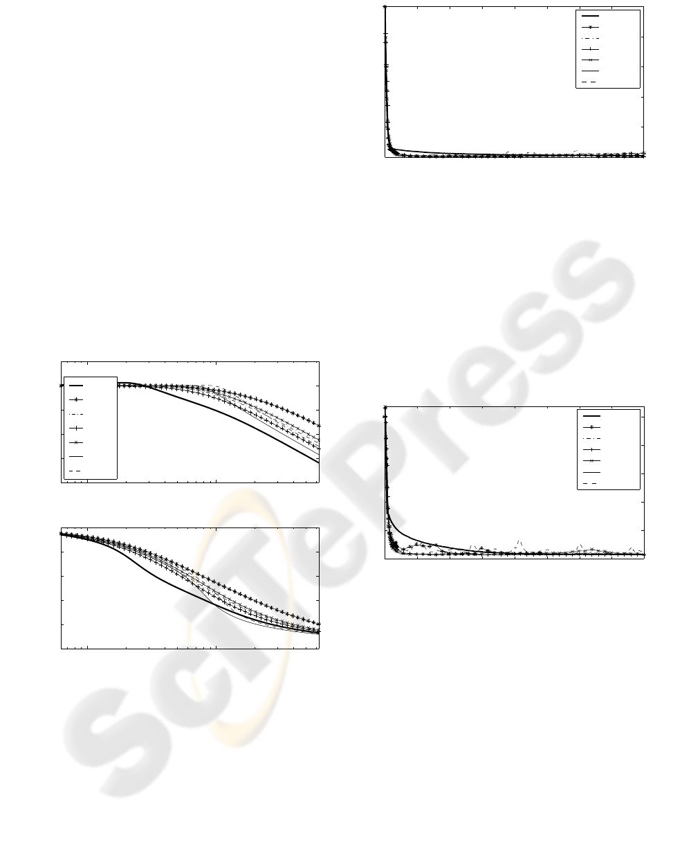
Figure 3 shows bode plots of six systems,
H
1
(jw) . . . H
6
(jw), resulting from applying the
state-feedback law (25) to the plant G(jw) for differ-
ent values of K. Each of these is in turn due to a
different choice of closed-loop pole locations. An op-
timisation routine was used to choose the pole loca-
tions in order to arrive at a flat magnitude plot with a
gain of 0 dB up until a prescribed cut-off frequency.
It was stipulated that H
1
(jw) and H
2
(jw) have com-
plex conjugate poles, H
3
(jw) and H
4
(jw) have real
poles, and H
5
(jw) and H
6
(jw) have a combination
and favour a sharper cut-off. The Bode plots asso-
ciated with these choices of pole locations show the
range of characteristic available to the designer. No
information relating to the phase of the systen has
been incorporated into the cost criteria for the op-
timisation. However the phase has been reduced at
low frequencies in each case and each system has an
IR that is either less than the period used or requires
negligible truncation. Therefore the problem of trun-
cation has been solved as a by-product of the design
process described. The systems H
1
(jw) . . . H
6
(jw)
10
0
10
1
−80
−60
−40
−20
0
20
Gain (dB)
Frequency (rad/s)
G(jw)
Φ
1
(jw)
Φ
2
(jw)
Φ
3
(jw)
Φ
4
(jw)
Φ
5
(jw)
Φ
6
(jw)
10
0
10
1
−500
−400
−300
−200
−100
0
Phase (degrees)
Figure 3: Bode plot of G(jw) and a variety of pole-placed
systems
are used with the adjoint algorithm, H
T
i
replacing G
T
e
in (7). Figure 4 shows the cycle error results for these
systems seen using the sine-wave demand. It is clear
that all the pole-placed systems lead to improved con-
vergence compared with G(jw) and there is no sign
of instability. Figure 5 shows cycle error results us-
ing the repeating sequence demand. The increased
bandwidth of this demand benefits from the increased
learning of the pole-placed systems compared to the
0 50 100 150 200 250 300 350
0
0.2
0.4
0.6
0.8
1
NE
Cycle No.
G(jw)
H
1
(jw)
H
2
(jw)
H
3
(jw)
H
4
(jw)
H
5
(jw)
H
6
(jw)
Figure 4: Cycle error for sine-wave demand
original. Only when using H
6
(jw), which has the
greatest bandwidth, are there signs of instability. It is
clear that robustness issues limit the frequencies that
can be learnt. Although the figure only shows results
from 400 cycles, the tests have been run for 1000 cy-
cles, with most of the pole-placed systems still show-
ing no sign of instability. This is a clear sign that their
convergence benefits over using G(jw) are not heav-
ily penalised in terms of lack of robustness. Figure 6
0 50 100 150 200 250 300 350
0
0.2
0.4
0.6
0.8
1
NE
Cycle No.
G(jw)
H
1
(jw)
H
2
(jw)
H
3
(jw)
H
4
(jw)
H
5
(jw)
H
6
(jw)
Figure 5: Cycle error for repeating sequence demand
highlights the initial convergence of the plant output
to the demand. It shows data from the 1
st
cycle and
every 5
th
thereafter. Excellent tracking is achieved
using the adjoint algorithm and H
5
(jw) by the 21
st
cycle compared to the slow convergence when using
G(jw) and the adjoint algorithm.
6 CONCLUSIONS AND FUTURE
WORK
This paper has explored the possibility of using a
well-know Iterative Learning Control algorithm in the
Repetitive Control framework. It has been noted that

0 5 10 15
−5
0
5
Output (rads)
Time (s)
Demand
H
5
(jw)
G (jw)
Figure 6: Tracking of repeating sequence demand
due to the non-causal nature of the algorithm, the al-
gorithm can be applied only to systems that have a
finite-impulse response (FIR). Furthermore, the im-
pulse response has to go to zero at most in N steps,
where N is period of the reference signal. If the plant
satisfies these assumptions, the tracking error con-
verges to zero exponentially.
If the plant does not satisfy the FIR assumption, the
algorithm can be still applied by using a plant model
where the impulse response is truncated after N time
steps. It turns out that if the phase of the multiplica-
tive uncertainty, which is caused by truncation, does
not exceed ±90 degrees, the algorithm still converges
exponentially to zero.
In the case when the uncertainty condition is not
met due to truncation, it is proposed that a dead-beat
controller can be used to shorten the length of the
impulse response. As a result, the closed loop sys-
tem should have an impulse response, which is short
enough for the algorithm to converge to zero tracking
error.
The algorithm has been applied to a non-minimum
phase spring-mass-damper system. The experimen-
tal results show that the algorithm is capable of pro-
ducing near perfect tracking after a small number of
cycles, demonstrating the algorithm should be appli-
cable to industrial problems.
The crucial point in tuning of the algorithm is the
selection of the feedback gain K. The objective is
to find a gain K that shortens the length of the im-
pulse response adequetely, produces rapid conver-
gence over the bandwidth and is robust. Currently K
is chosen using the ‘trial and error’ method. There-
fore, as a future work, it is important to find system-
atic design rules that can be used to tune K.
Another interesting future research topic is the tun-
ing of β. In ILC, it is possible to make β to be
iteration-varying, and it can be shown that it results in
enhances the robustness properties of the algorithm.
How to transfer this idea to RC framework is still an
open problem for future research.
ACKNOWLEDGEMENTS
J. Hätönen is supported by the EPSRC contract No
GR/R74239/01.
REFERENCES
Astrom, K. J. and Wittenmark, B. (1984). Computer Con-
trolled Systems: Theory and Design. Prentice-Hall.
Chen, K. and Longman, R. W. (2002). Stability issues us-
ing fir filtering in repetitive control. Advances in the
Astronautical Sciences, 206:1321–1339.
Francis, B. A. and Wonhan, W. M. (1975). The inter-
nal model principle for linear multivariable regulators.
Appl. Math. Opt., pages 107–194.
Freeman, C., Lewin, P., and Rogers, E. (2003a). Experi-
mental comparison of extended simple structure ILC
algorithms for a non-minimum phase plant. Submitted
to ASME.
Freeman, C., Lewin, P., and Rogers, E. (2003b). Experi-
mental evaluation of simple structure ILC algorithms
for non-minimum phase systems. Submitted to IEEE
Transactions on Mechatronics.
Fung, R. F., Huang, J. S., Chien, C. G., and Wang, Y. C.
(2000). Design and application of continuous time
controller for rotation mechanisms. International
journal of mechanical sciences, 42:1805–1819.
Garimella, S. S. and Srinivasan, K. (1996). Application
of repetitive control to eccentricity compensation in
rolling. Journal of dynamic systems measurement and
control-Transactions of the ASME, 118:657–664.
Hätönen, J., Owens, D. H., and Moore, K. L. (2003a). An
algebraic approach to iterative learning control. Inter-
national Journal of Control, 77(1):45–54.
Hätönen, J., Owens, D. H., and Ylinen, R. (2003b). A
new optimality based repetitive control algorithm for
discrete-time systems. In Proceedings of the Euro-
pean Control Conference (ECC03), Cambridge, UK.
Inouye, T., Nakano, M., Kubo, T., Matsumoto, S., and
Baba, H. (1981). High accuracy control of a proton
synchrotron magnet power supply. In Proceedings of
the 8th IFAC World Congress.
Kaneko, K. and Horowitz, R. (1997). Repetitive and adap-
tive control of robot manipulators with velocity es-
timation. IEEE Trans. on robotics and automation,
13:204–217.
Kobayashi, Y., Kimuara, T., and Yanabe, S. (1999). Robust
speed control of ultrasonic motor based on H
∞
con-
trol with repetitive compensator. JSME Int. Journal
Series C, 42:884–890.
Longman, R. W. (2000). Iterative learning control and
repetitive control for engineering practice. Interna-
tional Journal of Control, 73(10).