AN ACCURATE AND EFFICIENT PARAMETER
DECOUPLING FOR TRANSFER FUNCTION IDENTIFICATION
In-Yong Seo
Korea Electric Power Research Ins., 103-16 Munji,Yusung, Taejon,305-380, Korea
Allan E. Pearson
Department of Engineering, Brown University, Providence, RI 02912, USA
Keywords: Parameter decoupling, S
ystem identification, AWLS
Abstract: We present an improved parameter decoupling algorithm in estimating parameters
that characterize the
numerator and denominator of transfer function polynomials using the Adaptive Weighted Least Squares
arising (AWLS) and Weighted Least Squares (WLS) from Fourier moment functionals of the Shinbrot type.
This algorithm gives more accurate estimates and uses less computation than Pearson’s algorithm. Also,
simulation example shows that this algorithm can be applied for the frequency analysis of lightly damped
systems for which establishing steady state or stationary operation may require unreasonably long settling
times.
1 INTRODUCTION
A decoupling algorithm for optimal identification of
rational transfer function parameters of discrete-time
linear systems by least-squares (LS) fitting of
observed input/output (I/O) data sequences (Shaw,
1994) was provided. The numerator was estimated
by minimizing the optimization criterion, and using
the estimated numerator, the optimal denominator
was estimated by linear LS in one step. A decoupled
parameter estimation (DPE) algorithm for estimating
sinusoidal parameters from both 1-D and 2-D data
sequences corrupted by autoregressive (AR) noise
was presented (Li and Stoica, 1996). In the first step
of the DPE algorithm, a nonlinear LS criterion was
minimized by a relaxation algorithm to obtain the
sinusoidal parameters. These estimates were used in
the second step of the DPE algorithm, which
estimates the AR noise parameters by a linear LS
approach. A parameter decoupling method for
transfer function during quasi-harmonic operation
was proposed (Pearson, 1998) without any
simulation example. This presupposes a non-steady
state mode of operation over a single or integral
number of periods during which a sinusoidal input is
used as a probing signal. This deliberate use of a
sinusoid during an otherwise transient state of
system operation is motivated by the desire to
simplify the identification process via a parameter
decoupling that occurs in a particular frequency
domain model. We explored Pearson’s algorithm
with several simulation examples and improved its
estimation performance by a more accurate and
more effective method.
In contrast to (Pearson, 19
98), the use of a high
frequency sinusoid is proposed in the modified
alpha-stage to decouple the denominator parameters
(herein called alpha parameters). This makes it
possible to use lower indexed harmonic Fourier
series coefficients of the output than input harmonics
for the estimation of denominator parameters which
is advantageous because lower harmonics contain
more important information on the system. This
simple idea causes a huge difference in the
estimation performance of denominator parameters
and affects to the estimation of numerator
parameters through the weighting matrix in the beta-
stage which use alpha parameters.
Moreover, we propose to modify the bet
a-stage
by using a non-harmonic input for the probing
signal. By using non-harmonic input, one step
decoupling of numerator parameters (called beta
parameters) is possible, which decreases the
computation burden and increases estimation
performance compared to Pearson’s beta-stage.
160
Seo I. and Pearson A. (2004).
AN ACCURATE AND EFFICIENT PARAMETER DECOUPLING FOR TRANSFER FUNCTION IDENTIFICATION .
In Proceedings of the First International Conference on Informatics in Control, Automation and Robotics, pages 160-167
DOI: 10.5220/0001138001600167
Copyright
c
 SciTePress

Following a presentation of the models, the
decoupling procedures for the new algorithm is
delineated and the least squares identifiers and the
weighting matrixes for both stages in the modified
algorithm are formulated. Finally, the simulation
example is illustrated for the performance
comparison.
2 FREQUENCY DOMAIN MODEL
Consider a time-invariant, bounded-input bounded-
output stable linear differential system with scalar
input
and scalar output modeled on a
finite time interval [0,T] by the nth order differential
equation:
)(tu
)(ty
)/( dtdp =
(1)
∑∑∑
===
+=
n
j
j
j
n
j
j
j
n
j
j
j
tvpatupbtypa
b
000
)()()(
equivalently with operator polynomials
in
and with normalized to unity:
))(),(( pBpA
dtdp /=
0
a
, (2)
∑
=
+=
n
j
j
j
papA
1
1)(
∑
=
=
b
n
j
j
j
pbpB
0
)(
1)0(),()()()()()( =
+
= AtvpAtupBtypA
(3)
))(),(( tytu
denote an input/output data pair, and
denotes an additive-output white Gaussian noise
disturbance as defined by
)(tv
(4)
{} { }
)()()(,0)(
2
τδστ =+= tvtvEtvE
where
)(
τ
δ
is the Dirac delta function. Assuming
orders
of the polynomial pair
are specified with
, the problem is to estimate
the parameters
and ,
given noise-corrupted data truncated to a time
interval of length T. A “resolving frequency”
),(
b
nn
))(),(( sBsA
nn
b
≤
),...,,(
21 n
aaa ),...,,,(
210 nb
bbbb
0
ω
is
defined in relation to [0, T] by
T/2
0
π
ω
=
.
To introduce the Modulating Function
Technique (MFT), define a set of the nth order
complex Fourier type modulating function (Pearson,
1998):
n
titim
m
ee
T
t )1(
1
)(
00
−=
−− ωω
φ
(5)
,
Mm ,,1,0 L=
Tt
≤
≤0
where
0
ω
is the resolving frequency, T is the
time interval of the data block, and M is an integer
for controlling the highest frequency and number of
algebraic equations. Each
)(t
m
φ
satisfies the end
point conditions:
0|)(
0
=
=tm
k
tp φ
, , (6)
0|)( =
=Ttm
k
tp φ )1(,,1,0 −= nk L
Using the binomial expansion,
)(t
m
φ
can be
written as:
∑
=
+−
=
n
k
tkmi
km
ec
T
t
0
)(
0
1
)(
ω
φ
, (7)
⎟
⎟
⎠
⎞
⎜
⎜
⎝
⎛
−=
−
k
n
c
kn
k
)1(
Then define a Shinbrot-type moment functional
(Pearson, 1998) of order n given
on [0,T]:
)(tx
(8)
][
0
0
)()()( kmX
k
c
n
k
T
dttxt
m
x
m
f +
∑
=
=
∫
=
φ
where
is the Fourier coefficient of at
frequency
][kX
)(tx
0
ω
k
as shown in equation (11).
If
)
is any polynomial of degree n (or less) in
the differential operator
and if is
any n-times differentiable function on [0,T] or n-
times mean-square differentiable in the case of
stochastic signals, then as stated (Pearson, 1998):
(pP
dtdp /=
)(tx
(9)
∑
=
++=
n
k
km
kmXkmPcxpPf
0
][][))((
Equation (3) will be converted to the frequency
domain via the Shinbrot-type moment functionals of
order n in equation (9). The result is
mmm
Eccc
′
+
Γ
′
=
′
φ
,
},1,0{ L=
∈
Zm
(10)
where prime denotes the transpose of vector/matrix
and the following definitions apply:
),...,,(
10
′
=
n
cccc
,
⎟
⎟
⎠
⎞
⎜
⎜
⎝
⎛
−=
−
k
n
c
kn
k
)1(
⎥
⎥
⎥
⎥
⎥
⎦
⎤
⎢
⎢
⎢
⎢
⎢
⎣
⎡
+
+
=
⎥
⎥
⎥
⎥
⎥
⎦
⎤
⎢
⎢
⎢
⎢
⎢
⎣
⎡
+Γ
+Γ
Γ
=Γ
⎥
⎥
⎥
⎥
⎥
⎦
⎤
⎢
⎢
⎢
⎢
⎢
⎣
⎡
+
+
=
][
]1[
][
,
][
]1[
][
,
][
]1[
][
nmE
mE
mE
E
nm
m
m
nm
m
m
mmm
MMM
φ
φ
φ
φ
[
] ][][][ kYkAk = φ
,
[
] ][][][ kUkBk =Γ
,
][][][ kVkAkE =
and
(
)
][],[],[ kVkYkU
denote the kth harmonic
Fourier series coefficient triplet defined by
∫
−
=
T
tik
dtetvtytu
T
kVkYkU
0
0
))(),(),((
1
])[],[],[(
ω
(11)
In addition to the pair , it is assumed that
a bandwith
B
),(
b
nn
ω
is specified within which the user
will extract frequency components of the data to be
used in estimating the parameters. This means that
the following constraint applies if
is the highest
harmonic to be sought from the data using (11):
max
k
B
k
ω
ω
≤
0max
Assuming
is a bandlimited white noise
process with passband >
)(tv
BW
ω
, the equation error
is transformed to
)(tv
m
Ecm
′
=
)(
ε
,
Zm
∈
(12)
which is still zero-mean Gaussian.
The parameter decoupling and improvement of
estimation performance in parameter space for the
AN ACCURATE AND EFFICIENT PARAMETER DECOUPLING FOR TRANSFER FUNCTION IDENTIFICATION
161

model (10) is the main focus for the remainder of
this paper.
3 DECOUPLING THE ESTIMATE
Given the system bandwidth, a set of integers
is defined by
BW
M
BW
Z
{
}
BWBW
MZ ,,2,1 L=
such that the
frequencies
0
ω
ω
k
k
=
, represent
selected ‘knots’ at which to estimate the transfer
function
BW
Mk ,,2,1 L=
)()()(
kkk
iAiBiH
ω
ω
ω
=
,
1−=i
. The choice
of
is assumed to satisfy the equality:
BW
(13)
M
BWBW
nM ωω =+
0
)(
This need is based on the condition that the highest
frequency extracted from the data does not exceed
the bandwidth. The question of selecting an
appropriate
0
ω
and T is discussed later. Let an
be selected along with a complex number
such that the input signal
BW
Zm ∈
α
α
C
()
TttteCeC
T
tu
timtim
+≤≤+=
−
∗
αα
ω
α
ω
αα
αα
,
1
)(
00
(14)
represents the sinusoidal signal with amplitude of
TC /2
α
and frequency
0
ω
α
m
that is applied to the
system over a [0,T] time interval. However,
excitation of all modes on this interval is a necessary
condition to avoid degeneracy in estimating the
α
parameters. Corresponding to this choice, the jth
Fourier series coefficient from (11) for
is:
)(tu
α
[]
[
]
ααααα
δδ mjCmjCjU ++−=
∗
)(
(15)
where
denotes the discrete unit pulse.
[]
j δ
Substituting (15) into (10) gives
mmmmm
Eccc
′
+Γ=
′
−
αα
φ
, (16)
⎩
⎨
⎧
≥+−−
<
∈
nmformnmnm
nmform
m
αααα
αα
},,1,{
},,1,0{
L
L
where
α
, and have the same
definition as in (10) and their components are
defined by:
[]
αα
CmB
m
][=Γ
m
φ
m
E
[] ][][][ kYkAk
α
φ
=
, ,
[] ][][][ kUkBk
α
=Γ
][][][ kVkAkE =
where
represents the kth harmonic Fourier
series coefficient of the observed response
on [0,T] to the sinusoid (14) as computed from (11).
][kY
α
)(ty
α
In the modified algorithm, the least squares
formulations will focus on estimating the
parameters
1++
b
nn
{
}
b
nn
bbbaaa ,,,,,,,
1021
LL
in the transfer
function
α
θ
ω
ω
ω
ββ
][1
][
)(
)(
)(
k
k
k
k
k
m
mQ
iA
iB
iH
Λ+
==
, (17)
BWk
Zm ∈
)
,
)
,,,()(
2 n
ssss L=Λ
,,,,1()(
2
b
n
ssssQ L=
β
and the real-valued
α
and
β
θ
parameters are
defined by
),,,(
21
′
=
n
aaa L
α
,
),,,(
10
′
=
b
n
bbb L
β
θ
)(][
0
ω
kk
imm
Λ
=
Λ
,
α
ω
][1)(
0
kikA Λ
+
=
,
)(][
0
ω
ββ kk
imQmQ =
3.1 Modified Alpha Stage
In Pearson’s alpha-stage algorithm, the harmonics of
)1(
+
α
m
through were used for
regressor and regressand, and the lowest harmonic
which can be used is 2 when
. Because the
lower harmonics of the output, especially
fundamental, contain the more useful information of
the system, we propose to apply a high frequency
sinusoid and use lower indices of the Fourier series
coefficients than the value of
for the estimation
of the
)( nMm ++
αα
1=
α
m
α
m
α
parameters. To take advantages of low
index Fourier series coefficients, let us set
1
+
+
=
nMm
αα
(18)
where
is user a chosen frequency index in the
modified alpha-stage, and its recommended range is
shown in (19). i.e., apply a sinusoid with frequency
α
M
0
)1(
ω
α
+
+
nM
which is right above the bandwidth
and amplitude
TC /2
α
as a probing signal. With
this probing input, all low harmonics from DC to
)( nM
+
α
of the output data (which covers the
system bandwidth) can be used for the estimation of
the denominator by defining a new
, a set of
frequency index m values that makes the
α
Z
α
parameters decouple from the
β
θ
parameters in the
polynomial
, i.e., define
)(
k
iB ω
{
} ntonMwithMmmZ 42~0:
ααα
≤≤=
(19)
The
in the modified alpha-stage includes DC as
well as the fundamental. This is the major difference
between Pearson’s alpha-stage and the modified
alpha-stage.
α
Z
The one restriction which is sufficient to
facilitate the decoupling over the positive integers,
i.e., to ensure that
0
=
Γ
′
m
c
in (10), for the input
(14) with
in (18), is
α
m
α
mm
<
<
0
(20)
which will provide a total of
frequency
domain equations including the DC component.
1+
α
M
ICINCO 2004 - SIGNAL PROCESSING, SYSTEMS MODELING AND CONTROL
162

With
, the right side of (10) reduces to
α
Zm∈
m
Ec
′
and utilizing the relation
α
ω
][1)(
0
kikA Λ+=
it can
be rearranged as a linear regression on
α
.
, (21)
mmm
EcQcYc
′
+
′
−=
′
α
α
Zm∈
⎥
⎥
⎥
⎥
⎦
⎤
⎢
⎢
⎢
⎢
⎣
⎡
++
++
=
⎥
⎥
⎥
⎥
⎦
⎤
⎢
⎢
⎢
⎢
⎣
⎡
++Λ
++Λ
Λ
=
⎥
⎥
⎥
⎥
⎦
⎤
⎢
⎢
⎢
⎢
⎣
⎡
+
+
=
][][
]1[]1[
][][
,
][][
]1[]1[
][][
,
][
]1[
][
nmEnmA
mEmA
mVmA
Eand
nmYnm
mYm
mYm
Q
nmY
mY
mY
Y
mmm
MMM
To change the complex-valued regression model
into a real-valued column vector linear regression
model, an equivalent real-valued regression is
defined as follows:
(22)
Α
+−= εα
cc
QY
where the following notation applied for the
combined real and imaginary quantities:
⎥
⎥
⎥
⎥
⎥
⎥
⎥
⎥
⎥
⎥
⎥
⎦
⎤
⎢
⎢
⎢
⎢
⎢
⎢
⎢
⎢
⎢
⎢
⎢
⎣
⎡
′
′
′
′
′
′
=
⎥
⎥
⎥
⎥
⎥
⎥
⎥
⎥
⎥
⎥
⎥
⎦
⎤
⎢
⎢
⎢
⎢
⎢
⎢
⎢
⎢
⎢
⎢
⎢
⎣
⎡
′
′
′
′
′
′
=
⎥
⎥
⎥
⎥
⎥
⎥
⎥
⎥
⎥
⎥
⎥
⎦
⎤
⎢
⎢
⎢
⎢
⎢
⎢
⎢
⎢
⎢
⎢
⎢
⎣
⎡
′
′
′
′
′
′
=
Α
α
α
α
α
α
α
ε
M
M
M
M
c
M
M
c
Ec
Ec
Ec
Ec
Ec
Ec
Qc
Qc
Qc
Qc
Qc
Qc
Q
Yc
Yc
Yc
Yc
Yc
Yc
Y
Im
Im
Im
Re
Re
Re
,
Im
Im
Im
Re
Re
Re
,
Im
Im
Im
Re
Re
Re
1
0
1
0
1
0
1
0
1
0
1
0
M
M
M
M
M
M
)1(2 +
ℜ∈
α
M
c
Y
, and
nM
c
Q
×+
ℜ∈
)22(
α
)1(2 +
Α
ℜ∈
α
ε
M
Note that the row dimension of
, and
c
Y
c
Q
Α
ε
is
. Based on this regression model and
assuming linearly independent regressors and zero-
mean Gaussian residuals
)1(2 +
α
M
Α
ε
with a nonsingular
covariance matrix
{
}
ΑΑ
′
=
ε
ε
α
EW
, a weighted least
squares estimate is defined by
(23)
cccc
YWQQWQ
1
1
1
ˆ
−
−
− ′
⎟
⎠
⎞
⎜
⎝
⎛
′
−=
αα
α
where
α
is a symmetric positive definite
weighting matrix.
W
Moreover,
α
ˆ
can be estimated by the iterative
method (Shen, 1993), which can be expressed by the
following equation:
, (24)
()
c
k
cc
k
ck
YWQQWQ
1
1
,
1
1
1
,
ˆ
−
−
−
−
−
′′
−=
αα
α
L,2,1=k
where
1
denotes the covariance matrix of the
residual vector, which will be shown in equation
(41), as a function of unknown parameter
,
−k
W
α
α
θ
and
evaluated at the previous iterate
1, −k α
θ
. Thus
)(
1,1, −−
=
kk
WW
ααα
θ
. But the initial weighting matrix
is taken as the identity matrix.
0, α
W
3.2 Weighting Matrix in the Modified
Alpha Stage
The composite residual vector
Α
ε
can be expressed
as follows
(25)
⎥
⎦
⎤
⎢
⎣
⎡
=
⎥
⎦
⎤
⎢
⎣
⎡
=
Α
I
R
α
α
α
α
ε
ε
ε
ε
ε
Im
Re
and the following definitions apply:
⎥
⎥
⎥
⎥
⎦
⎤
⎢
⎢
⎢
⎢
⎣
⎡
=
][
]1[
]0[
αα
α
α
α
ε
ε
ε
ε
M
M
⎥
⎥
⎥
⎥
⎦
⎤
⎢
⎢
⎢
⎢
⎣
⎡
++
++
=
][][
]1[]1[
][][
nmVnmA
mVmA
mVmA
E
m
M
m
Ecm
′
=][
α
ε
Equivalent vector-matrix representation for
is
α
ε
(26)
αααα
ε VPC=
where matrix
, diagonal matrix , and vector
are given by
α
C
α
P
α
V
⎥
⎥
⎥
⎥
⎦
⎤
⎢
⎢
⎢
⎢
⎣
⎡
=
n
n
n
ccc
ccc
ccc
C
LL
OOOM
LL
LL
10
10
10
00
0
000
000
α
])[],...,1[],0[( nMAAAdiagP +=
αα
)][],...,1[],0[(
′
+= nMVVVV
αα
α
C
is a real matrix defined by
sequentially moving the row vector
c
over one
entry to the right with 0’s elsewhere, as shown
above,
is complex with
)1()1( ++×+ nMM
αα
′
α
P
)(][
0
ω
imAmA =
and
is a complex valued column vector. The covariance
matrix for the
α
V
)12(
+
α
M
dimensional residual vector
Α
ε
will have the block diagonal structure:
(27)
{}
⎥
⎥
⎦
⎤
⎢
⎢
⎣
⎡
Θ
Θ
=
′
=
ΑΑ
)(
)(
a
I
a
R
W
W
EW
θ
θ
εε
α
α
α
where
{
}
{
}
']0[
2
)()(
11
2
2
0
2
eeAcCPPCEW
HRRR
+
′
=
′
=
αααααααα
σ
εεθ
(28)
{
}
{
}
']0[
2
)()(
11
2
2
0
2
eeAcCPPCEW
HIII
−
′
=
′
=
αααααααα
σ
εεθ
(29)
in which
)][,,]1[,]0[(
22
2
nMAAAdiagPP
H
+=
α
L
,
2
0
2
)(][ ω imAmA =
,
1]0[
=
A
, is a zero matrix and
superscript H denotes conjugate transpose. Unit
column vector
is given by in which
Θ
1
e
)1(
11
′
Θ=
×
α
n
e
α
n×
Θ
1
is a zero vector with a dimension of
α
.
n×1
3.3 Modified Beta Stage
Pearson’s beta-stage algorithm needs another
computation step to extract the
parameters from
the number
i
b
(
)
{
} 2/1+
b
nceil
of algebraic equations
where the function ceil(A) rounds the elements of A
AN ACCURATE AND EFFICIENT PARAMETER DECOUPLING FOR TRANSFER FUNCTION IDENTIFICATION
163

to the nearest integer greater than or equal to A..
Moreover, his algorithm needs
times
of the weighting matrix inversion computation in the
beta-stage. This inconvenience was eventually
caused by the harmonic operation in the beta-stage.
Since the extracted parameter
’s are inversely
proportional to
, as will be shown in (38), and
the resolving frequency
(){ 2/1+
b
nceil }
i
b
i
0
ω
0
ω
is usually a small
number for high resolution, less than 1, the bias and
standard deviation of
’s are amplified. This
problem is inevitable as long as the indirect
parameter estimation algorithm, which uses
harmonic sinusoids for a probing signal is adopted in
the beta-stage. To improve the problems of
inconvenience and inaccuracy in estimating the
numerator parameters with Pearson’s beta-stage
algorithm, the modified beta-stage is proposed,
which estimates numerator parameters at one shot
using non-harmonic operation.
i
b
Again, assume that an estimate
α
ˆ
has been
obtained following the completion of the modified
alpha-stage as described in the previous section, and
consider a non-harmonic sinusoidal input,
)
, like
a sweep sine, as a probing signal in the modified
beta-stage. To ensure the excitation of all modes, a
sweep sine with Fourier coefficients, which covers
the system bandwidth, should be chosen. The model
(10) is changed by:
(tu
β
(30)
mmm
Eccc
′
+
′
=
′
β
θγφ
where the following definitions apply:
and
),...,,(
10
′
=
n
cccc
),,,(
10
′
=
b
n
bbb L
β
θ
⎥
⎥
⎥
⎥
⎦
⎤
⎢
⎢
⎢
⎢
⎣
⎡
+
+
=
⎥
⎥
⎥
⎥
⎦
⎤
⎢
⎢
⎢
⎢
⎣
⎡
+
+
=
⎥
⎥
⎥
⎥
⎦
⎤
⎢
⎢
⎢
⎢
⎣
⎡
+
+
=
][
]1[
][
,
][
]1[
][
,
][
]1[
][
nmE
mE
mE
Eand
nm
m
m
nm
m
m
mmm
MMM
γ
γ
γ
γ
φ
φ
φ
φ
, ,
[]
][][
ˆ
][ kYkAk = φ
[] ][][][ kUkQk
ββ
γ =
][][
ˆ
][ kVkAkE =
),,,,1()(
2
b
n
ssssQ L=
β
,
)(][
0
ω
ββ
ikQkQ =
,
β
Zm∈
where the following definition apply:
(31)
}0:{
ββ
MmmZ ≤≤=
where
is explained in (32). In equation (30),
]
denotes the kth harmonic Fourier coefficient
of the input
on
β
M
[kU
β
)(tu
β
Tt ≤
≤
0
. Note that in
(17) was separated into two terms,
and
][kB
][kQ
β
β
θ
,
in order to estimate the
parameters directly.
There are
parameters to be estimated. Let
denote a user-selected integer used to
specify the number of frequency indices upon which
to base the estimate of
’s. Choose
i
b
1+
b
n
1+≥
b
nM
β
i
b
)1(4)1(2
+
+
≈
bb
ntonM
β
. (32)
To change the complex-valued regression model
into a real-valued column vector linear regression
model, define combined constituents by
Β
+
Φ
=
ε
θ
ξ
β
(33)
where the following notation applies for the
combined real and imaginary quantities:
⎥
⎥
⎥
⎥
⎥
⎥
⎥
⎥
⎥
⎥
⎥
⎦
⎤
⎢
⎢
⎢
⎢
⎢
⎢
⎢
⎢
⎢
⎢
⎢
⎣
⎡
′
′
′
′
′
′
=
⎥
⎥
⎥
⎥
⎥
⎥
⎥
⎥
⎥
⎥
⎥
⎦
⎤
⎢
⎢
⎢
⎢
⎢
⎢
⎢
⎢
⎢
⎢
⎢
⎣
⎡
′
′
′
′
′
′
=Φ
⎥
⎥
⎥
⎥
⎥
⎥
⎥
⎥
⎥
⎥
⎥
⎦
⎤
⎢
⎢
⎢
⎢
⎢
⎢
⎢
⎢
⎢
⎢
⎢
⎣
⎡
′
′
′
′
′
′
=
Β
β
β
β
β
β
β
ε
γ
γ
γ
γ
γ
γ
φ
φ
φ
φ
φ
φ
ξ
M
M
M
M
M
M
Ec
Ec
Ec
Ec
Ec
Ec
c
c
c
c
c
c
c
c
c
c
c
c
Im
Im
Im
Re
Re
Re
,
Im
Im
Im
Re
Re
Re
,
Im
Im
Im
Re
Re
Re
1
0
1
0
1
0
1
0
1
0
1
0
M
M
M
M
M
M
, and
)1(2 +
ℜ∈
β
ξ
M
b
nM ×+
ℜ∈Φ
)22(
β
)1(2 +
Β
ℜ∈
β
ε
M
Note that the row dimension of
ξ
, and
Φ
Β
ε
is
)1(2
+
β
M
. Based on this regression model and
assuming linearly independent regressors and zero-
mean Gaussian residuals
with a nonsingular
covariance matrix
Β
ε
{
}
ΒΒ
′
=
ε
ε
β
EW
, the estimate of
β
θ
can be obtained by
(
)
ξθ
βββ
1
1
1
ˆ
−
−
−
′
ΦΦ
′
Φ= WW
(34)
Note that
is estimated by the Weighted Least
Squares (WLS) using the
β
θ
ˆ
α
ˆ
estimates, which is
accurately estimated in the modified alpha-stage.
3.4 Weighting Matrix in the Modified
Beta Stage
If we follow the same procedure in section 3.2, we
get the block diagonal covariance matrix for the
)1(2
+
β
M
dimensional residual vector
Β
ε
in the
modified beta-stage:
⎥
⎥
⎦
⎤
⎢
⎢
⎣
⎡
′
−
′
Θ
Θ
′
+
′
=
11
2
2
0
11
2
2
0
2
]0[
ˆ
]0[
ˆ
2
eeAcCPPC
eeAcCPPC
W
H
H
ββββ
ββββ
β
σ
(35)
where
)][
ˆ
,,]1[
ˆ
,]0[
ˆ
(
22
2
nMAAAdiagPP
H
+=
βββ
L
,
2
0
2
)(
ˆ
][
ˆ
ω imAmA =
and
. is a real
matrix which has the same pattern as (26) and
is
a function of parameter
1]0[
ˆ
=A
β
C
)1()1( ++×+ nMM
ββ
β
P
α
ˆ
, which is estimated in the
modified alpha-stage. Note that the weighting
matrix for the modified beta-stage,
, needs to be
computed only once to estimate the
numerator
parameters.
β
W
i
b
ICINCO 2004 - SIGNAL PROCESSING, SYSTEMS MODELING AND CONTROL
164

3.5 Selection of
0
ω
with Modified
Algorithm
The highest harmonics required of the output data
over the data intervals
[
]
and
Ttt +
αα
,
[
]
Ttt
+
ββ
,
, are
the
th and
)
th harmonics respectively,
cf. (22) and (33). For a strictly proper rational
transfer function, i.e.,
, and assuming the
same ratio for the selection of
and in
((19), (32)) is chosen, then
is bigger than
and the corresponding highest frequency is
)( nM +
α
( nM +
β
b
nn >
α
M
β
M
)( nM +
α
)( nM +
β
0
)(
ω
α
nM +
. It follows that
0
ω
should be chosen as
)(
0
nM
BW
+
=
α
ω
ω
(36)
With this choice, both frequency models in (22) and
(33) cover the system bandwidth
BW
ω
. Also, this
choice assures adherence to the equality (20) made
earlier as a condition on selecting
.
BW
M
All modes of a system might not be exited by a
low frequency sinusoid as used in Pearson’s alpha
stage algorithm. But by applying this one sinusoid
with a frequency that is just outside bandwidth, all
high frequency system information within the
system bandwidth could be obtained. This is another
great advantage of the modified algorithm.
4 SIMULATION RESULTS
An 8
th
order system with 4th-order in the numerator,
as shown in the following, was used to evaluate and
compare the performance of the Pearson’s
decoupling algorithm (Pearson, 1998) and the
modified decoupling algorithm devised in this study:
)8.001.0)(5.001.0)(3002.0)(2.103.0(
1.0452
)(
234
isisisis
ssss
sH
±+±+±+±+
++++
=
(37)
For the above specific system, its step response
will take about 400 seconds to reach steady state,
which is a lightly damped case. The data were
collected during the system transient state, mostly
during the first 50 sec. The system bandwidth is 3.38
. 2048 data of input/output were sampled
for T sec, where T varies with
in each
algorithm.
sec]/[rad
α
m
Fig. 1 shows the Bode diagram of the system
used for simulation. The noise-to-signal ratio (NSR),
which characterizes the percent additive noise on the
output is defined as
Bode Diagram
Frequency (rad/sec)
Phase (deg) Magnitude (dB)
−80
−60
−40
−20
0
20
40
H(s)=(s
4
+2s
3
+5s
2
+4s+0.1)
/(s+0.03±j1.2)(s+0.002±j3)(s+0.01±j0.5)(s+0.01±j0.8)
10
−3
10
−2
10
−1
10
0
10
1
−540
−360
−180
0
180
Figure 1: Bode diagram of the system
%100.
)(
)(
)]([
)]([
%100
2
0
2
0
2
0
0
2
ty
tn
dtty
dttn
NSR
T
T
==
∫
∫
where
is a noise free signal, and is an
additive noise sequence. As for a true parameter
)(
0
ty
)(tn
j
θ
,
its ensemble average
and the number of
parameters L, a composite normalized bias error
(CNB) and standard deviation (CNSTD) are defined
as:
j
θ
ˆ
CNB =
%
ˆ
1
1
2
∑
=
⎟
⎟
⎠
⎞
⎜
⎜
⎝
⎛
−
L
j
j
jj
L θ
θθ
CNSTD =
%
1
1
2
∑
=
⎟
⎟
⎠
⎞
⎜
⎜
⎝
⎛
L
j
j
j
L θ
σ
where
j
σ
is the standard deviation of the estimate
of the true
j
θ
. These will be used to measure the
accuracy of the different algorithms.
In Pearson’s algorithm, we used the routine
SOLVE in Symbolic Math Toolbox of MATLAB to
solve the algebraic equations for the extraction of
’s parameters in the numerator from beta
parameters,
i
b
)(Re][
0
ωβ
kk
R
imBm =
, , .
)(Im][
0
ωβ
kk
I
imBm =
L,2,1=k
For instance, 5
’s of the example system in
equation (37) are shown;
i
b
)3(
10
1
)2(
5
3
)(
2
3
0000
ωβωβωβ
RRR
b +−=
0
00
1
6
)2()(8
ω
ωβωβ
II
b
−
=
2
0
000
2
24
)3(3)2(16)(13
ω
ωβωβωβ
RRR
b
+−
=
(38)
3
0
00
3
6
)2()(2
ω
ωβωβ
II
b
−
=
4
0
000
4
120
)3(3)2(8)(5
ω
ωβωβωβ
RRR
b
+−
=
Note that the parameter
’s are inversely
proportional to
, and is usually a small
number for high resolution. Thus the computed
’s
from the
i
b
i
0
ω
0
ω
i
b
β
’s have wide distribution. This is the
AN ACCURATE AND EFFICIENT PARAMETER DECOUPLING FOR TRANSFER FUNCTION IDENTIFICATION
165

reason why Pearson’s beta-stage produces large
composite STD. This is the disadvantage of “Quasi-
Harmonic operation”. To improve this large STD
problem, the modified beta-stage is suggested with a
simulation example in the next section.
In this section, we will compare the modified
decoupling algorithm denoted by
αβ
MOD
, which
uses the modified alpha-stage and modified beta-
stage, with Pearson’s algorithm, denoted by HAR,
and an intermediate algorithm denoted by
α
MOD
,
which uses the modified alpha-stage and Pearson’s
beta-stage. In the experiment setup, we focus on
adding the same noise level for the different
algorithms. The system bandwidth
BW
ω
is 3.38
and the sampling rate is around 45 Hz.
500 Monte Carlo runs were made for each NSR
under the initial condition fixed at zeros. Here we
will explain simulation setups for three different
algorithms.
sec]/[rad
1) Input parameters for the Pearson’s algorithm:
For the estimation of denominator parameters in the
alpha-stage,
, and
11 jC +=
α
1=
α
m
162
=
=
nM
α
were chosen, so
0.1352
0
=
ω
and the
observation time interval is
[sec], and
was used for a probing signal
in the alpha-stage. For the estimation of numerator
parameters in the beta-stage, three harmonics were
applied to the system one by one to estimate 3 sets
of
sec]/[rad
46.47=T
titi
eCeCtu
00
)(
ω
α
ω
αα
−
∗
+=
β
parameters and they are given
by:
, ,
.
titi
eCeCtu
00
)(
1
ω
α
ω
αβ
−
∗
+=
titi
eCeCtu
00
22
2
)(
ω
α
ω
αβ
−
∗
+=
titi
eCeCtu
00
33
3
)(
ω
α
ω
αβ
−
∗
+=
2) Input parameters for the
α
MOD
algorithm:
25=
α
m
, and were chosen,
so the probing signal in the modified alpha-stage is
. For the beta-stage, the
same 3 harmonic inputs as in Pearson’s beta-stage
were used.
and
162 == nM
α
11 jC +=
α
titi
eCeCtu
00
2525
)(
ω
α
ω
αα
−
∗
+=
0.1408
0
= ω
sec]/[rad
44.61
=
T
were used both in the alpha and beta stage.
Notice that
and T are a little different with those
of Pearson’s algorithm [4] because the computation
methods of
for both algorithms are different.
[sec]
0
ω
0
ω
3) Input parameters for the
αβ
MOD
algorithm:
Here,
,
25=
α
m
162
=
= nM
α
and were
chosen, and
was applied
for the modified alpha-stage and
11 jC +=
α
titi
eCeCtu
00
2525
)(
ω
α
ω
αα
−
∗
+=
(
)
75
sin1119.0)(
2
t
tu =
β
for the modified beta-stage, which produced the
same output norm as
to ensure the same level
of noise can be added in the alpha and beta stage.
)(tu
α
0
2
4
6
0
5
10
15
20
NSR(%)
Composite Bias(%)
(a) Composite Bias of DEN
HAR
MODα
MODαβ
0
2
4
6
0
5
10
15
20
25
NSR(%)
Composite STD(%)
(b) Composite STD of DEN
HAR
MODα
MODαβ
0
2
4
6
0
20
40
60
80
100
120
NSR(%)
Composite Bias(%)
(c) Composite Bias of NUM
HAR
MODα
MODαβ
0
2
4
6
0
20
40
60
80
100
120
140
NSR(%)
Composite STD(%)
(d) Composite STD of NUM
HAR
MODα
MODαβ
0
2
4
6
0
20
40
60
80
100
NSR(%)
Composite Bias(%)
(e) Composite Bias of DEN and NUM
HAR
MODα
MODαβ
0
2
4
6
0
20
40
60
80
100
NSR(%)
Composite STD(%)
(f) Composite STD of DEN and NUM
HAR
MODα
MODαβ
Figure 2: CNB and CNSTD of Pearson’s algorithm and
the modified algorithm
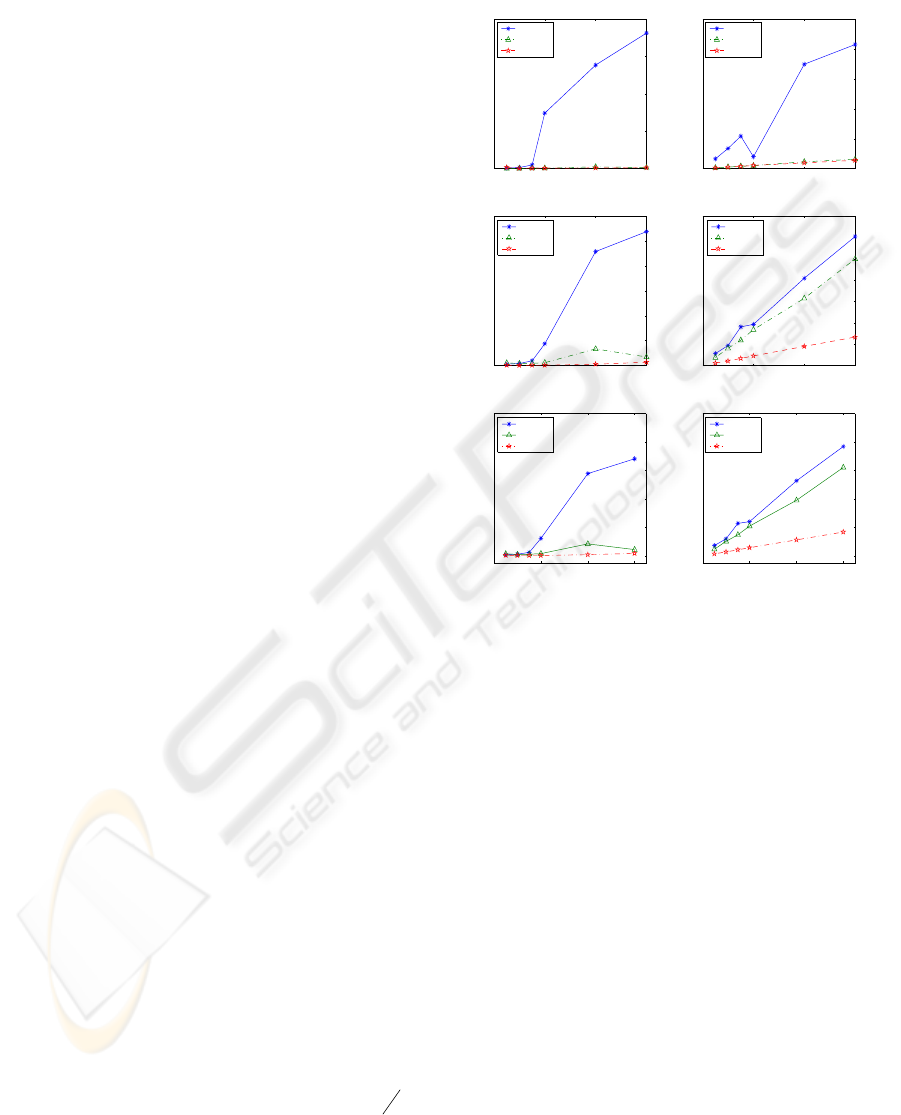
Fig. 2 shows the composite bias and STD for
three different algorithms. For the composite bias of
the denominator shown in Fig. 2(a), the bias for
Pearson’s algorithm is as small as that for the
modified alpha-stage algorithm when the NSR is
less than 1.5 %, but the composite bias and
composite STD of the denominator sharply increase
to 17% and 21%, respectively, as the NSR increases
from 2% to 6%. In other words, Pearson’s alpha-
stage algorithm is very sensitive to noise.
The composite biases and the composite STDs of the
denominator for
α
MOD
and
αβ
MOD
are almost
the same because they both use the modified alpha-
stage algorithm, see Fig. 2(a) and (b). The modified
alpha-stage shows excellent performance over the
Pearson’s alpha-stage. The
α
MOD
shows better
performance than Pearson’s algorithm in beta-stage
even though the two algorithms use the same
Pearson’s beta-stage. That results from the fact that
the
α
MOD
uses a weighting matrix in Pearson’s
beta-stage based on the accurately estimated
denominator parameters by the modified alpha-
ICINCO 2004 - SIGNAL PROCESSING, SYSTEMS MODELING AND CONTROL
166

stage. The composite bias of the numerator was
greatly reduced by the
α
MOD
, but the composite
STD of the numerator was not much improved by
the
α
MOD
, see Fig. 2(c) and (d). In Fig. 2(c) and
(d), the
αβ
MOD
shows better performance for the
numerator than the
α
MOD
both in composite bias
and composite STD aspects. This means that the
modified beta-stage improves not only standard
deviation but also bias. The composite bias of the
numerator for Pearson’s algorithm is very large as
we expected. But it is greatly reduced by the
modified beta-stage algorithm. Even though the
modified beta-stage algorithm reduces the composite
bias and composite STD of the numerator, those
values are larger than the denominator’s.
From Fig. 2(a) ~ (d), we can know that both the
modified alpha-stage and modified beta-stage
algorithm have decreased the bias and standard
deviation at each NSR. Fig. 2(e) and (f) show the
composite bias and composite STD of all parameters
including the denominator and numerator. The
αβ
MOD
, the proposed algorithm, produces the
lowest bias and standard deviation among the three
algorithms.
5 CONCLUDING REMARKS
We have presented a new parameter decoupling
algorithm for the transfer function identification on
the basis of Pearson’s algorithm using harmonic and
non-harmonic signals. We have also shown with
simulation examples that these algorithms offer
significant improvement in estimation performance
and computation burden over existing methods.
In the new algorithm, we apply a harmonic
sinusoid with one high frequency component outside
the system bandwidth in the alpha-stage, so that we
can use the lower indexed Fourier coefficients for
the denominator estimation. Also, a one step
estimation algorithm was adopted using a sweep sine
input as probing signal for the numerator parameters
in beta-stage. By using one step estimation
algorithm, the computation burden was decreased
and the estimation performance was increased.
Clearly, simulation results show that the modified
parameter decoupling algorithm is much better than
Pearson’s algorithm.
REFERENCES
Shaw A. K., 1994. A Decoupled Approach for Optimal
Estimation of Transfer Function Parameters from
Input-Output Data.
IEEE Trans. on Signal Processing,
vol. 42, no. 5, pp. 1275-1278.
Li J. and Stoica P., 1996. Efficient Mixed-Spectrum
Estimation with Applications to Target Feature
Extraction.
IEEE Trans. on Signal Processing, vol. 44,
no. 2, pp. 281-295.
moderstroS
&&&&
T. and Stoica P., 1989. System Identification,
Prentice Hall International Ltd.
Pearson A. E., 1998. Parameter Decoupling for Transfer
Function Identification During Quasi-Harmonic
Operation.
Proc. of 1998 American Control Conf., vol.
5, pp. 3607-3611.
Pearson A. E. and Shen Y., 1993. Weighted Least
Squares/MFT algorithms for linear differential System
Identification.
Proc. 32
nd
Conference on Decision and
Control
vol. 7, pp. 2032-2037.
Pearson A. E., 1999. Frequency Domain Scaling
Strategies for Linear Differential System
Identification.
Proc. of European Control Conf. Paper
No. F1013-4.
Shen Y., 1993.
System Identification and Model Reduction
Using Modulating Function Technique
. Ph.D. thesis,
Division of Engineering, Brown University,
Providence, Rhode Island.
Symbolic Math Toolbox, Version 2.1.2. The Math Works,
Inc.
AN ACCURATE AND EFFICIENT PARAMETER DECOUPLING FOR TRANSFER FUNCTION IDENTIFICATION
167