
INTERACTIVE SOFTWARE FOR SYMBOLIC MODELING OF
PHYSICAL SYSTEMS USING GRAPHS
André Laurindo Maitelli
DCA – LECA – UFRN, CEP 59072–970, Natal/RN, Brazil
Gilbert Azevedo da Silva
GEINF – CEFET/RN, CEP 59015–000, Natal/RN, Brazil
Keywords: CAD/CAM, Control Education, System Modeling, Graph, Symbolic Transfer Function, Mason´s Rule.
Abstract: This paper presents a computational environment for teaching of control systems: Modsym. The software
implements a graphical interface for physical systems modeling using graphs and calculates systems transfer
functions in symbolic form. ModSym generalizes elements and dynamics variables of some physical
systems based on the energy concept. This approach allows to represent and to connect elements of different
systems in a linear graph. An algorithm implemented in the software, also presented in this paper, obtain a
signal flow graph for the system linear graph which makes possible to use the Mason’s rule in calculating of
the system transfer function.
1 INTRODUCTION
Control Engineering studies the physical systems
dynamics. The most important activities of this
engineering are modeling, analysis, simulation,
design, implementation and verification of physical
systems, (Kroumov and Inoue, 2001). The modeling
activity is an especially important step of the system
dynamics study. In this step, a mathematical model
for the system is proposed. The other activities are
realized based on this model. So, it is important to
define a model that represents the system dynamics.
The modeling activity demands a great effort of
control students. In modeling of a system, they have
to study the dynamics of each system element and to
analyze all connections between them. Due to this
hard task, a lot of control students have difficulties
in formulating and solving the system equations that
result from modeling process. So, computational
tools are frequently used as an aid to the educational
process of control courses. The information and
communication technologies have been widely
discussed in Pedagogy, (Quartiero, 1999), and in
Control Engineering, (Dorf and Bishop, 1999). A
great number of educators are also evaluating the
future directions in control education in face of the
new technologies related to this area, (Heck 1999).
However, despite the progress in computational
science, most of computers software related to
control system area is poor in the educational
process. An analysis of some available tools has
shown that these ones present a not suitable man-
machine interface. In general, they are based on
command interaction, which makes the work tedious
and difficulties the learning process, (Kroumov and
Inoue, 2001).
In this reality, this paper presents ModSym, a
computational tool for symbolic modeling of
physical systems. The software allows to model
systems of several physical domains using liner
graphs. The software aid the educational process in
control area and its purpose is to calculate system
transfer functions in symbolic form.
In modeling of physical systems, ModSym
implements an interactive and easy-to-use graphical
interface that allows connecting elements like
sources, dissipaters, stores, transformers and energy
couplers. When connections are done, the software
allows the students to calculate, step by step, the
system transfer function (STF). An important step of
this process is the generation of a signal-flow graph
(SFG) for the system. In particular, the algorithm
that makes this task is also a contribution of this
paper.
488
Laurindo Maitelli A. and Azevedo da Silva G. (2004).
INTERACTIVE SOFTWARE FOR SYMBOLIC MODELING OF PHYSICAL SYSTEMS USING GRAPHS.
In Proceedings of the First International Conference on Informatics in Control, Automation and Robotics, pages 488-491
DOI: 10.5220/0001138404880491
Copyright
c
SciTePress
2 SYSTEM MODELING
2.1 Generalized Variables
The idea of systems as energy handling devices is
essential to modeling process using linear graphs,
(Wellstead, 1979). The energy concept implicates in
defining two generalized variables: effort and flow,
whose purpose is identify the similarities that exist
over some physical systems. The effort variable
represents a physical variable that is measured
across two distinct points of the system and the flow
variable is measured through only one system point.
The physical elements are thought of as energy
manipulators, which interact with inputs and outputs
via “energy ports”. The energetic interactions that
occur through these ports determinate just how and
in what sense energy are transmitted inside the
system. The elements are so classified in according
to number of energy ports and energy process. One-
port basic elements can be classified as sources:
effort sources (E) and flow sources (F); stores: effort
stores (ES) and flow stores (FS); and dissipaters
(ED). Two-port elements can be classified as
transformers, gyrators and couplers. Table 1 presents
generalized variables and elements for mechanical,
electrical and fluid systems.
Table 1: Generalized Variables and System Elements
System Mechanical Fluid Electrical
Effort
Velocity
v / w
Pressure
P
Voltage
V
Flow
Force/Torque
F / T
Flow
Q
Current
I
ES
Spring
K
Fluid Inductor
L
F
Inductor
L
FS
Mass / Inertia
M / J
F. Capacitor
C
F
Capacitor
C
ED
Damper
B
Fluid Resistor
R
F
Resistor
R
2.2 Linear Graphs
The Network Method is one way to systemize
physical system modeling, (Wellstead, 1979). This
method uses generalized variables and system
elements to represent a system as an oriented graph
usually known as linear graph. The graph nodes
represent points of common effort and the edges
represent the system elements.
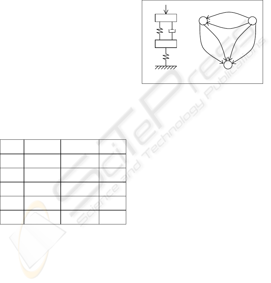
Figure 1a shows a simplified, quarter-body car
suspension. The suspension is modeled as a mass M
1
representing the mass of the wheel and other
components located between the leaf spring and the
road. This mass is coupled to the road through
spring K
1
that represents tire elasticity. The mass M
2
contains the car frame, car body and all components
within the body. It is connected to M
1
through spring
K
2
and damper B
1
that represent the leaf spring and
shock absorber of the suspension, (Durfee et al.,
1991).
(a) (b)
K
1
M
1
F
B
1
M
2
K
2
3
2
1
K
1
-1
S
B
1
-1
K
2
-1
S
F
M
1
-1
S
-1
M
2
-1
S
-1
3
1
2
Figure 1: Car Suspension Example
Figure 1b contains the linear graph for the
example. The reference and masses define the points
of common velocities that are indicated by the nodes
1 to 3. The passive elements - masses, springs and
damper - and the active element that indicates the
force F are represented by edges. All edges have a
gain given by constitutive property of the element
that describe its physical characteristics.
The constitutive properties and inter-connective
constraints on system elements can be used to obtain
a mathematical model for the system. With them,
ModSym generate a SFG for the physical system and
uses this new graph to calculate the system transfer
function using Mason’s rule (Mason, 1956).
3 MODSYM
The current version of ModSym implements two
graphical interfaces for physical system modeling:
one for linear graphs and other for signal-flow
graphs. A third interface with graphical components
will be present in a new version. This interface shall
allow users to model physical systems connecting
graphical components that represent electrical,
mechanical, fluid, thermal and magnetic elements.
3.1 Linear Graph Interface
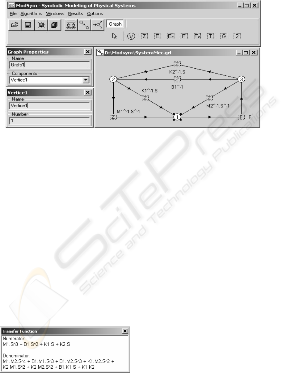
The linear graph interface, shown in figure 2, allow
to model systems with nine types of graphical
components: 1 − node or vertex (V): linear graph
INTERACTIVE SOFTWARE FOR SYMBOLIC MODELING OF PHYSICAL SYSTEMS USING GRAPHS
489
node that represent common effort points;
2 − impedance (Z): passive one-port element that
represents energy stores and dissipaters; 3 − effort
source (E): energy source with a defined effort;
4 − controlled effort source (Ec): energy source with
effort controlled by a system variable; 5 − flow
source (F): energy source with a defined flow;
6 − controlled flow source (Fc): energy source with
flow controlled by a system variable;
7 − transformer (T): two-port element that act like
ideal transformer; 8 − gyrator (G): two-port element
that act like ideal gyrator and 9 − generic two-port
element (2).
The components palette shown at ModSym main
window aid users to select and add elements at the
system. Properties windows shown beside the graph
are used to define names, gains and elements
connections.
For calculating the system transfer function
(STF), the users have to select the its input and
output variables. Input variables must be a system
excitation and output variables can be the effort or
flow variable in any system element. The figure 3
shows a transfer function for the car suspension
example. The input and output variables were the
force F applied to the system and the velocity of the
mass M
2
, respectively.
Figure 3: STF for Car Suspension Example
3.2 Signal-Flow Graph Interface
The software interface for system modeling with
SFG is very similar to the interface previously
shown. It allows to model systems with two types of
graphical components: 1 − variables (V): graph
nodes that represent the signal-flow variables and
2 − transmittances (T): Graph edges that represent
the relations between those variables.
The SFG interface works in the same way of the
linear graph one.
3.3 Algorithm: Linear Graph to SFG
The algorithm linear graph to signal-flow graph
implemented at ModSym systematizes the generation
of SFG of physical systems. The aim is to use
computational algorithms, like Mason’s rule, to
obtain systems transfer functions in symbolic form.
The first algorithm step is the determination of
signal-flow graph variables. These variables are
given by effort and flow variables at all physical
system elements. So, each physical element
contributes with two SFG variables: the effort at the
element and the flow through it.
In the next step, the constitutive proprieties and
and inter-connective constraints of the system linear
graph are used to generate a equation system in
symbolic form. This system gives the relation
between the physical system excitations and the
generalized variables of the system elements.
Finally, a deep search algorithm is used to find
functions that associate each equation system
variable with the another variables. These functions
are used to determinate the SFG transmitances.
Figure 2: Linear Graph Interface
ICINCO 2004 - ROBOTICS AND AUTOMATION
490
4 EXAMPLE
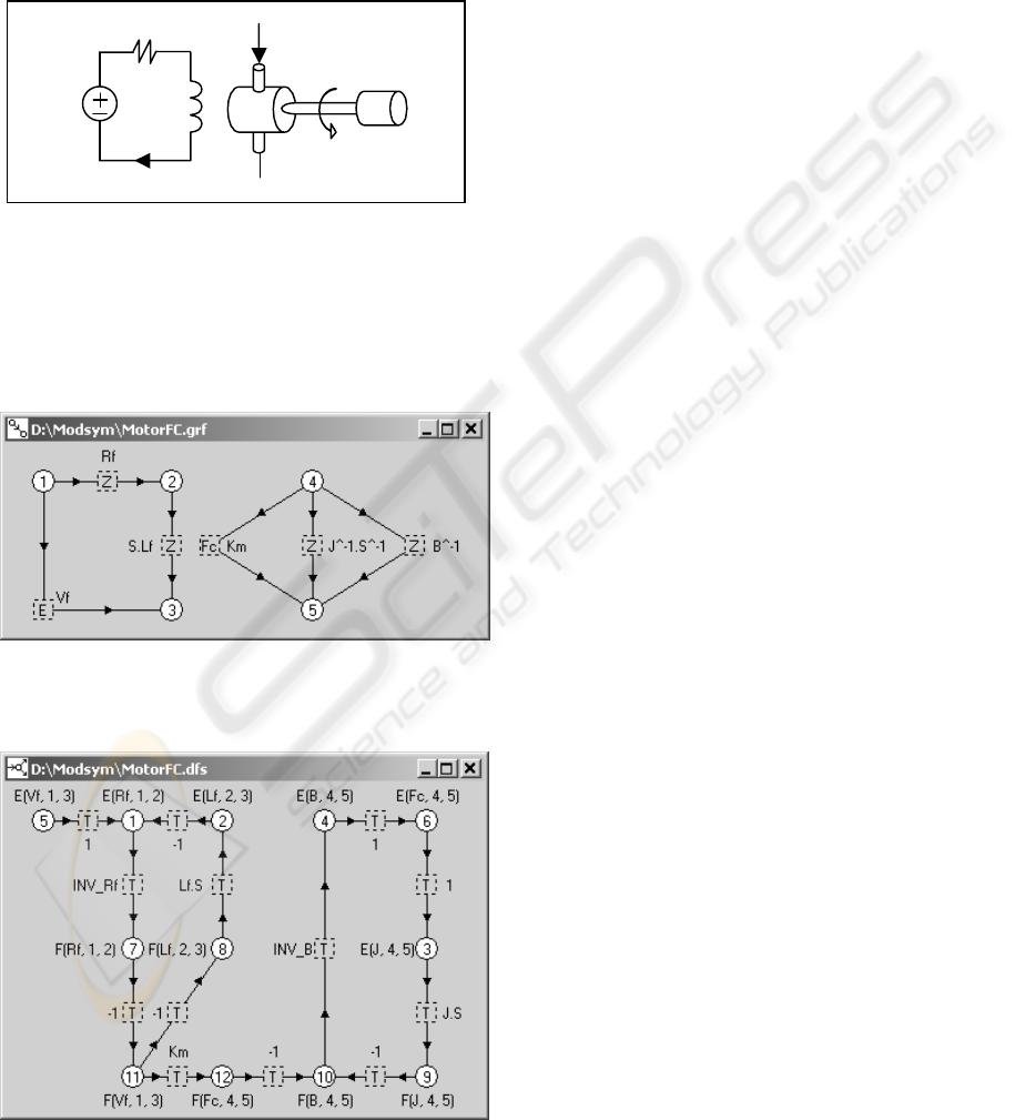
4.1 Field Controlled DC Motor
Figure 4 shows a model for a field controlled DC
motor, (Dorf and Bishop, 1995). The motor converts
direct current electrical energy into rotational
mechanical energy, which is applied to a load.
R
f
V
f
L
f
I
f
J, B
I
a
W
Figure 4: Field Controlled DC Motor
Figure 5 shows the linear graph for DC motor.
An effort source represents the voltage source.
Generalized impedances represent the load and
electrical resistance and inductance. A controlled
flow source with gain K
m
proportional to field
current I
f
represents the motor.
Figure 5: Linear Graph for DC Motor
The SFG generated by algorithm is shown in
figure 6.
Figure 6: SFG for DC Motor
5 CONCLUSIONS
The software ModSym, presented in this paper, is a
very interesting tool for education in control and
related areas. The software can be used to solve
practical problems and to aid students in learning of
control theory.
In laboratories, the software is powerful in
physical system modeling and can aid students to
project systems and to obtain mathematical models.
The calculus of systems transfer functions that is
essential to several systems manipulations as
simulations and optimizations can be done with
precision and quickness.
In education process, the software can be used in
several courses like control, physics, mechanical an
electrical systems. The graphical resources of the
software that allow to model systems using linear
and signal-flow graphs can be used to produce high
quality educational texts. Moreover, the software
can be used to study a wide range of control systems
that aren’t available in laboratories.
REFERENCES
Dorf, R.C. and R.H. Bishop. 1995. Modern Control
Systems Addison-Wesley, MA, USA.
Dorf, R.C. & R.H. Bishop. 1999. “Teaching Modern
Control System Design”.
Proc. of the 38th IEEE
Conference on Decision and Control, Vol. 1 , pp. 364
–369.
Durfee, W.K., M.B. Wall, D. Rowell & F.K. Abbott.
1991. “Interactive Software for Dynamic System
Modeling Using Linear Graphs”.
IEEE Control
Systems Magazine
, Vol. 11(4), pp. 60-66.
Heck, B.S. 1999. “Future Directions in Control
Education”.
IEEE Control Systems Magazine, Vol.
19(5), pp. 16-17.
Kroumov, V. & H. Inoue. 2001. “Enhancing Education in
Automatic Control via Interactive Learning Tools”.
Proc. of the 40th SICE Annual Conference, pp. 220-
225.
Mason, S.J. 1956. “Feedback Theory – Further Properties
of Signal-Flow Graphs”.
Proc. IRE, Vol. 44, pp. 920-
926.
Quartiero, E.M. 1999. “As Tecnologias da Informação e
Comunicação e a Educação”.
Revista Brasileira de
Informática na Educação, Nº. 4, pp. 69-74.
Wellstead, P.E. 1979.
Introduction to Physical System
Modelling. Academic Press, London.
INTERACTIVE SOFTWARE FOR SYMBOLIC MODELING OF PHYSICAL SYSTEMS USING GRAPHS
491
