POSITION AND ORIENTATION CONTROL OF A TWO-WHEELED

DIFFERENTIALLY DRIVEN NONHOLONOMIC MOBILE ROBOT

Frederico C. Vieira Adelardo A. D. Medeiros Pablo J. Alsina Ant

onio P. Ara

ujo Jr.

Federal University of Rio Grande do Norte – Departament of Computer Engineering and Automation

UFRN-CT-DCA – Campus Universit

ario – 59072-970 Natal RN Brazil

Keywords:

Nonholonomic robots, robot control, stabilization control, linear modeling of robots.

Abstract:

This paper addresses the dynamic stabilization problem of a two-wheeled differentially driven nonholonomic

mobile robot. The proposed strategy is based on changing the robot control variables from x, y and θ to

s and θ, where s represents the robot linear displacement. Using this model, the nonholonomic constraints

disappear and we show how the linear control theory can be used to design the robot controllers. This control

strategy only needs the robot localization (x, y, θ), not requiring any velocity measurement or estimation. The

complete derivation of the control strategy and some simulated results are presented.

1 INTRODUCTION

There are many feedback controllers proposed in the

literature (Aicardi et al., 1995; d’Andrea Novel et al.,

1995; Lizarralde, 1998; Samson, 1993; Tanner and

Kyriakopoulos, 2002; Yang and Kim, 1999) for non-

holonomic wheeled mobile robots. Most of these

strategies only deal with the problem of kinematic

compensation (Aicardi et al., 1995; d’Andrea Novel

et al., 1995; Samson, 1993). Pure kinematic con-

trollers lie on the simpliﬁcation that the generated

control signal is instantaneously applied to the robot

actuators, not taking into account the dynamic effects.

Recently, some control strategies have been pro-

posed to deal with dynamic compensation of mobile

robots (Lages and Hemerly, 2000; Lizarralde, 1998;

Tanner and Kyriakopoulos, 2002). Most of them are

derived via Lyapunov techniques and do not present

a correspondence between the controller parameters

and the robot dynamic behavior. Many of the dy-

namic control laws also requires the measurement of

the robot velocities, not always accurate or available.

The control strategy proposed on this paper ad-

dresses the dynamic compensation of mobile robots

and only requires information about the robot local-

ization. The problem classiﬁcation is presented on

section 2 and the kinematic and dynamic model of

the considered robot, on section 3. The control sys-

tem design is presented on section 4 and some results

and ﬁnal considerations, on sections 5 and 6.

2 PROBLEM CLASSIFICATION

There are two main problems in mobile robots con-

trol: the trajectory tracking problem and the stabilisa-

tion problem.

The stabilisation problem states that the robot must

reach a desired conﬁguration (x

, y

and θ

) start-

ing from a given initial conﬁguration (x

, y

and θ

)

(Luca et al., 1998). This control problem is also

known as a parking problem. There are several feed-

back controllers proposed in the literature for the sta-

bilisation problem (Aicardi et al., 1995; Lizarralde,

1998; Tanner and Kyriakopoulos, 2002), some of

them with the previously presented limitations.

In the trajectory tracking problem, the robot must

reach and follow a trajectory in the Cartesian space

starting from a given initial conﬁguration (Luca et al.,

1998). There are several feedback controllers pro-

posed in the literature that address only the trajectory

tracking problem (Oliveira and Lages, 2001; Samson,

1993; Yang and Kim, 1999).

The trajectory tracking problem is simpler than the

stabilisation problem because there is no need to con-

trol the robot orientation: it is automatically compen-

sated as the robot follows the trajectory, provided that

the speciﬁed trajectory respects the non-holonomic

constraints of the robot. As the control strategy pre-

sented in this paper is concerned with the stabilisation

problem, it can also be applied to the trajectory track-

ing problem.

256

Vieira F., Medeiros A., Alsina P. and Araújo Jr. A. (2004).

POSITION AND ORIENTATION CONTROL OF A TWO-WHEELED DIFFERENTIALLY DRIVEN NONHOLONOMIC MOBILE ROBOT.

In Proceedings of the First International Conference on Informatics in Control, Automation and Robotics, pages 256-262

DOI: 10.5220/0001138702560262

 SciTePress

3 MODELLING

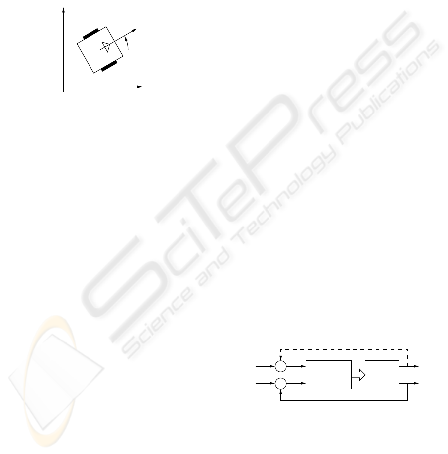
A schematic diagram of the considered robot is pre-

sented on ﬁgure 1. The robot conﬁguration is repre-

sented by its position on the Cartesian space (x and y,

that is the position of the robot-body center with re-

lation to a referential frame ﬁxed on the workspace),

and by its orientation θ (angle between the robot ori-

entation vector and the reference axis – X, ﬁxed on

the workspace).

θ,ω

Figure 1: Schematic diagram of a two-wheeled nonholo-

nomic robot.

The kinematic model represents the movements

constraints of the robot body. For the considered

robot, the kinematic model is given by equation 1.

q =





˙x

˙y





cos(θ) 0

sin(θ) 0

0 1

= G(θ)·v (1)

The vector q = [

x y θ

]

represents the linear

and angular positions and the vector v = [

v ω

]

represents the linear and angular velocities. The main

feature of this model for wheeled mobile robots is

the presence of nonholonomic constraints, due to the

rolling without slipping condition between the wheels

and the ground. The nonholonomic constraints im-

pose that the system generalized velocities ( ˙x, ˙y and

θ) cannot assume independent values. It can be ob-

served that the kinematic model in equation 1 does

not include the dynamic effects of the robot body and

actuators.

The dynamic model is derived from the actua-

tors dynamics and the robot dynamics parameters,

like mass, inertia momentum and friction coefﬁcients.

The ﬁnal dynamic model for a robot with two DC

motors directly connected to the wheels (Yamamoto

et al., 2003) is given by equation 2:

Ku = M ˙v + Bv (2)

The vector u = [

]

represents the input sig-

nals, usually currents or tensions applied to the left

and right electrical motors of the robot. K is a gain

matrix that transforms the input signals u into forces

to be generated by the robot wheels. M is the gener-

alized inertia matrix and B is the generalized viscous

friction matrix.

The model in equation 2 is a multi-variable lin-

ear system and a simple control law for the dynamic

stabilisation problem could be designed. However,

two drawbacks can be highlighted: the measurement

of the state variables (v and ω) is usually inaccurate

or unavailable, and velocities references are not well

suited for the mobile robot stabilisation control prob-

lem, where the references are usually coordinates on

the Cartesian space and an orientation angle.

Models in equations 1 and 2 can be rearranged into

a single state space representation, by deﬁning the

matrices

A = −M

−1

B and

B = M

−1







. 0

. . . . . . . . .

G(θ)

. 0











. .





u (3)

The outputs in equation 3 are x, y and θ. Although

this model allows the use of Cartesian coordinates and

orientation angles as references to the mobile robot,

it is a multi-variable non-linear model and the devel-

opment of control laws based on such model is not

trivial.

In order to reduce the model complexity, one could

rewrite it in terms of the robot linear and angular dis-

placement, s and θ, so that ˙s = v and

θ = ω. Deﬁning

a vector p = [

s θ

]







. 0

. . . . . .

. 0











. .





u (4)

The model in equation 4 is linear, with outputs s

and θ. One could easily design a control system based

on the block diagram on ﬁgure 2, if s and θ are mea-

surable and s

ref

and θ

ref

are deﬁned. This controller

can be based on any of the classic design techniques

for linear systems where the controller receives the er-

ror signal and generates the input to the plant (a PID,

for example).

Controller Robot

−

ref

Figure 2: Control system block diagram.

As the design of such a controller is simple, this

model has been used for the control system design,

despite of two problems that still hold: the linear dis-

placement s along a trajectory is practically unmea-

surable and s

ref

is meaningless. However, these prob-

lems can be contoured, as will be shown on the next

section.

POSITION AND ORIENTATION CONTROL OF A TWO-WHEELED DIFFERENTIALLY DRIVEN

NONHOLONOMIC MOBILE ROBOT

257

4 CONTROL SYSTEM DESIGN

The robot stabilisation problem can be divided into

two different control problems: robot positioning

control and robot orientating control. The robot po-

sitioning control must assure the achievement of a de-

sired position (x

ref

, y

ref

), regardless of the robot ori-

entation. The robot orientating control must assure

the achievement of the desired position and orienta-

tion (x

, y

, θ

4.1 Robot positioning control

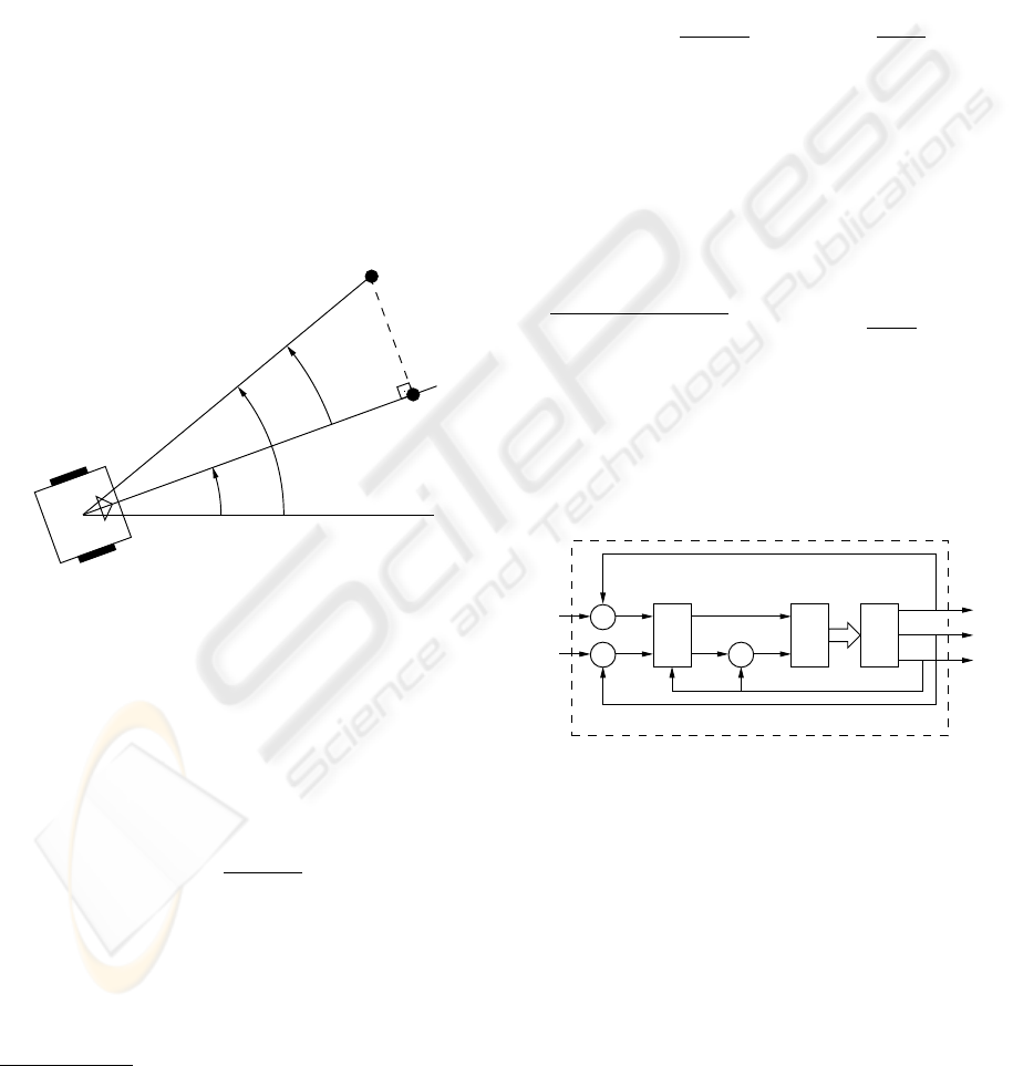
Figure 3 illustrates the positioning problem, where ∆l

is the distance between the robot and the desired ref-

erence (x

ref

, y

ref

) in the Cartesian space. The robot

positioning control problem will be solved if we as-

sure ∆l → 0. This is not trivial since the l variable do

not appear in the model of equation 4.

∆φ

ref

, y

ref

)

∆λ

∆l

(x, y)

Figure 3: Robot positioning problem

To overcome this problem, we can deﬁne two new

variables, ∆λ and φ. ∆λ is the distance to R, the

nearest point from the desired reference that lies on

the robot orientation line; φ is the angle of the vector

that binds the robot position to the desired reference.

We can also deﬁne ∆φ as the difference between the

φ angle and the robot orientation: ∆φ = φ − θ.

We can now easily conclude that:

∆l =

∆λ

cos(∆φ)

(5)

So, if ∆λ → 0 and ∆φ → 0 then ∆l → 0. That is,

if we design a control system that assures the ∆λ and

∆φ convergence to zero

, then the desired reference,

ref

and y

ref

, is achieved. Thus, the robot positioning

control problem can be solved by applying any con-

trol strategy that assures such convergence.

It is not even necessary to assure the convergence

of ∆φ to zero: the convergence to any ∆φ value where

cos(∆φ) 6= 0 will be acceptable.

The block diagram in ﬁgure 2 suggests that the sys-

tem can be controlled using linear and angular ref-

erences, s

ref

and θ

ref

, respectively. We will generate

these references in order to ensure the converge of ∆λ

and ∆φ to zero, as required by equation 5. In other

words, we want e

= ∆λ and e

= ∆φ. Thus, if the

controller assures the errors convergence to zero, the

robot positioning control problem is solved.

To make e

= ∆φ, we just need to deﬁne θ

ref

= φ,

so e

= θ

ref

− θ = φ − θ = ∆φ. For this, we make:

ref

= tan

−1

ref

− y

ref

− x

= tan

−1

∆y

ref

∆x

ref

(6)

To calculate e

is generally not very simple, be-

cause the s output signal cannot be measured and we

cannot easily calculate a suitable value for s

ref

. But

if we deﬁne the R point in ﬁgure 3 as the reference

point for the s controller, only in this case it is true

that e

= s

ref

− s = ∆λ. So:

= ∆λ = ∆l · cos(∆φ) = (7)

(∆x

ref

)

+ (∆y

ref

)

· cos

tan

−1

∆y

ref

∆x

ref

− θ

The complete robot positioning controller, based

on the diagram of ﬁgure 2 and the equations 6 and 7, is

presented on ﬁgure 4. It can be used as a stand-alone

robot control system if the problem is just to drive to

robot to a given position (x

ref

, y

ref

), regardless of the

ﬁnal robot orientation.

−

Positioning control system

Controller Robot

ref

, θ

ref

Calcul of

Figure 4: Robot positioning controller

4.1.1 Practical aspects

The Brockett’s theorem (Brockett, 1983; Stern, 2002)

proved that no continuous control law can completely

stabilize a system with the non-holonomic restriction

as in equation 1. The best any such control law can

do is to drive the system to a region delimited by a

circle of radius as small as posible around the desired

ﬁnal position. This restriction naturally appears in the

control law proposed in this article: it is impossible to

calculate the angular reference θ

ref

in equation 6 when

the robot reaches the position reference (x

ref

, y

ref

). To

ICINCO 2004 - ROBOTICS AND AUTOMATION

258

deal with this limitation, we deﬁne, based on the pre-

cision of the position measurement sensors, an ac-

ceptable distance error (²). When the robot enters this

circular region (∆l < ²), the angular error e

and the

linear error e

are assumed to be zero.

The angular error e

should be normalized to the

interval −π/2 ≤ e

≤ π/2. When the robot is near

the sign change border (e

≈ ±π/2), it is sometimes

better to slightly exceed the ±π/2 limit to maintain

the sign of the angular error the same of the previ-

ous iteration. This avoids unnecessary changes in the

direction of the angular movement.

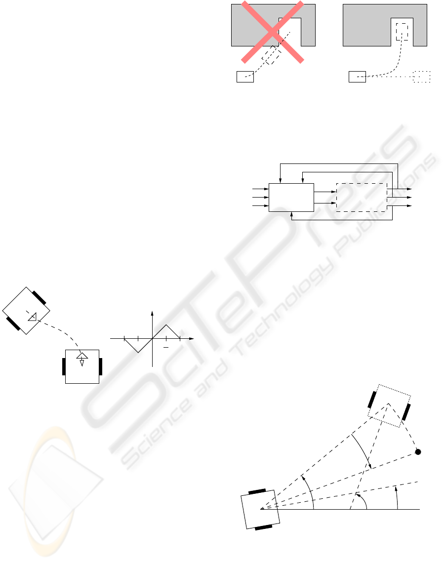
Only allowing values between −π/2 and π/2 for

the angular error does not favor forward movements,

as illustrated by the ﬁrst trajectory in ﬁgure 5. But if

the robot cannot move as better in the backward di-

rection as in the forward one, the second trajectory in

ﬁgure 5 would be preferable in some situations. To

obtain this behavior, the angular error e

should be

restricted to the interval −π ≤ e

≤ π. The ±π lim-

its for the angular error can only be applied when the

robot is far enough from the desired reference point.

If they are applied when the robot is near the ﬁnal po-

sition, small overshots can make the robot indeﬁnitely

turn around the reference point.

Figure 5: Forward and backward movements

4.2 Robot orientating control

The main idea behind the proposed orientating con-

trol strategy is that when we want to move to a ﬁnal

position with a ﬁxed orientation, it is not usually a

good idea to go straight to this position, as illustrated

by ﬁgure 6. Generally, we drive as if we wanted to

go to another place until a moment where, if we go

straight to the ﬁnal position, we will reach it with the

desired orientation.

In order to attend the robot orientating control

problem, an external loop with a moving reference

scheme has been designed. The external loop gener-

ates Cartesian references, x

ref

and y

ref

, for the internal

loop (the positioning control scheme), such that the

robot reaches the desired position (x

and y

) with the

desired orientation (θ

). This approach is illustrated

Figure 6: The orientating control idea

on ﬁgure 7: the positioning controller block can be

the one presented on ﬁgure 4 or any other one.

Positioning

controller

reference

Moving

generator

ref

Figure 7: Dynamic stabilisation controller

The strategy to calculate the internal reference is

presented on ﬁgure 8. The reference (x

ref

, y

ref

) is cal-

culated by rotating the vector of length ∆d pointing

from the robot position to the desired position by an

angle of γ. Practical aspects of calculating γ will be

discussed latter, but it is essentially equal to the dif-

ference between the desired ﬁnal orientation (θ

) and

the angle to move to the desired position (β):

γ = β − θ

(8)

(x, y)

, y

)

θθ

ref

, y

ref

)

∆d

Figure 8: Robot orientating problem

If β and θ

coincide, γ = 0 and the robot goes

straight to the ﬁnal position (x

ref

, y

ref

) = (x

, y

). If

not, as long as the robot tries to move to the internal

reference (x

ref

, y

ref

), the difference between θ

and β

raises, γ decreases and (x

ref

, y

ref

) tends to (x

, y

POSITION AND ORIENTATION CONTROL OF A TWO-WHEELED DIFFERENTIALLY DRIVEN

NONHOLONOMIC MOBILE ROBOT

259

The moving reference scheme is so driven by the

following equations:

ref

= x + ∆d · cos (β − γ)

ref

= y + ∆d · sin (β − γ)

(9)

where x and y are the robot Cartesian coordinates, θ

is the desired orientation, and ∆d and β are presented

on ﬁgure 8:

∆d =

− x)

+ (y

− y)

(∆x

)

+ (∆y

)

β = tan

−1

− y

− x

= tan

−1

∆y

∆x

(10)

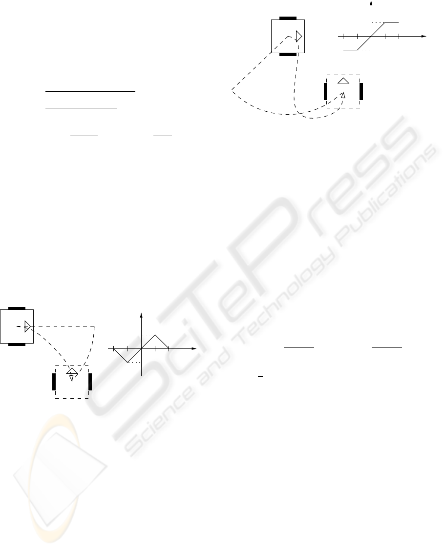
4.2.1 Practical aspects

The γ angle in equation 8 should be restrained to the

interval −π/2 ≤ γ ≤ π/2. The speciﬁc way to do

this restriction depends on the robot capabilities.

If the robot can move as well in one direction as in

the order, it is irrelevant if the robot reaches the de-

sired orientation with or without a rotation of π. In

the example of ﬁgure 9, we want a ﬁnal orientation

= π/2, but the robot ﬁnished the mouvement with

an orientation of θ

= −π/2. This behavior (bidi-

rectional orientation) is achieved by normalizing the

γ angle, as illustrated by the graphic in ﬁgure 9.

= π/2

ref

, y

ref

β = −π/4

γ = π/4

π/2

−π/2

−π

β − θ

Figure 9: Bidirectional orientation

Sometimes a non-inversed ﬁnal orientation is re-

quired. In this case (unidirectional orientation), the γ

angle should be saturated (and not normalized), as il-

lustrated by the graphic in ﬁgure 10. This orientating

control strategy should be combined with a position

control strategies that favors forward mouvements, as

described in section 4.1.1. The limitation of this kind

of position control (see 4.1.1) imposes that the unidi-

recional orientating control strategy can only be ap-

plied when the robot is far enough from the desired

reference point.

4.3 The linear controller

The controller appearing on ﬁgures 2 and 4 can be

designed using any of the classical control techniques

γ = −π/2

β = −π/4

ref

, y

ref

π/2

−π/2

β − θ

−π

= π/2

Figure 10: Unidirectional orientation

that can be used with a linear multi-variable system

described by the model in equation 4. We will ex-

emplify with a simple controller based on decoupled

PIDs, but in no way it should be assumed that the con-

trol strategy presented on sections 4.1 and 4.2 must

necessarily be used with a PID-based controller.

If the robot is symmetrical and driven by two iden-

tical DC motors, the K, M and B matrices in equa-

tion 2 have the following properties (Yamamoto et al.,

2003):

K =

α α

β −β

M, B are diagonals

We can deﬁne two new input signals, v

and v

and

a new input vector w = [

]

such that:

+ u

− u

w =

1 1

1 −1

u ⇒ u =

1 1

1 −1

w (11)

If we introduce the new w input vector in equa-

tion 4 and calcute the transfer model equivalent to the

space stade equation, we obtain a decoupled system:

S(s)

Θ(s)

(s) 0

0 G

(s)

(12)

Using equation 12, it is very simple to design two

independent PID controllers for s and θ, based on the

desired linear and angular behavior. The output of

these controllers are the virtual input signals v

and

: to calculate the real input signals u

and u

, we

use equation 11.

5 RESULTS

Simulated results of the proposed strategy are pre-

sented on this section. A simple PD controller has

been implemented as the positioning controller. The

ICINCO 2004 - ROBOTICS AND AUTOMATION

260

robot dynamic model has been derived via experimen-

tal identiﬁcation of a real mobile robot (Guerra et al.,

2004).

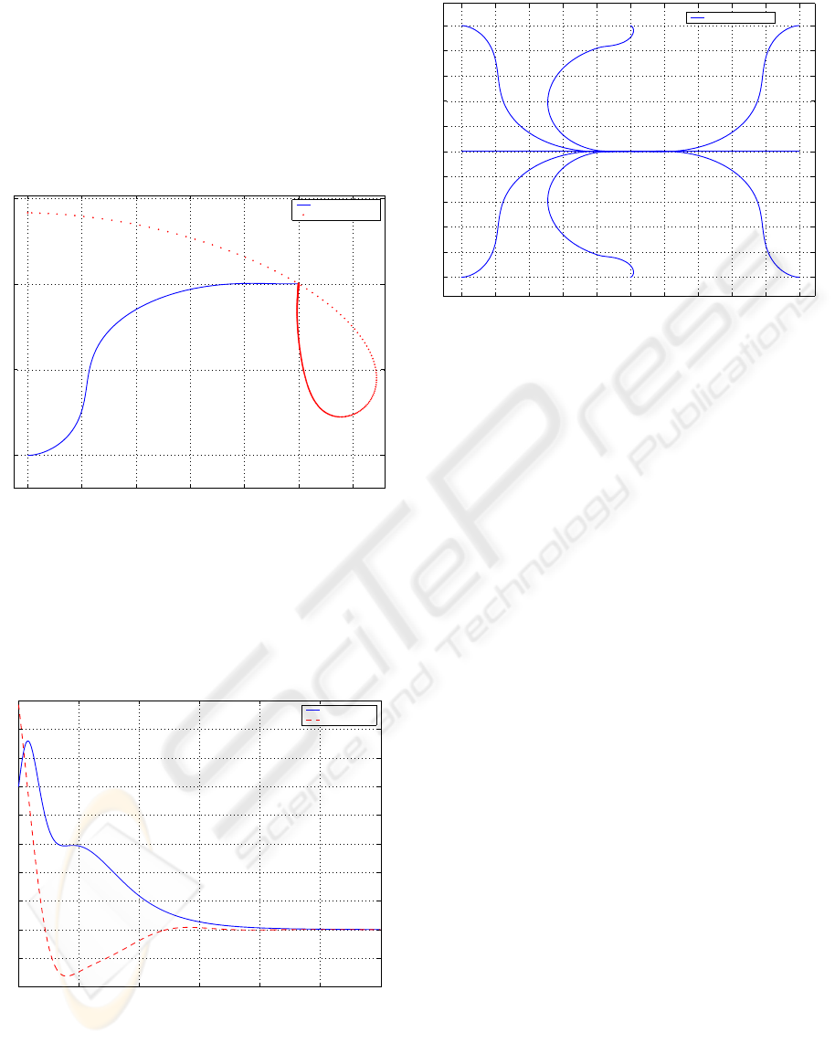
On ﬁgure 11 a simulation for the robot stabilisation

control problem is shown, where the initial conditions

are x = 0, y = 0 and θ = 0, and the desired conﬁg-

uration is x

= 1, y

= 1 and θ

= 0. The moving

reference scheme can also be observed on ﬁgure 11.

0 0.2 0.4 0.6 0.8 1 1.2

0.5

1.5

Robot Trajectory

Reference

Figure 11: Mobile robot stabilisation.

Figure 12 shows the linear and angular errors con-

vergence to zero, thus, assuring the achievement of

the control objective. It must be noticed that the con-

troller performance can be improved through the PD

gains adjustment.

0 5 10 15 20 25 30

−0.4

−0.2

0.2

0.4

0.6

0.8

1.2

1.4

1.6

time (seconds)

Linear Error

Angular Error

Figure 12: Linear and angular errors for the robot stabilisa-

tion simulation.

On ﬁgure 13 a set of simulations with the same ﬁnal

conﬁguration (x = 0, y = 0 and θ = 0) and different

initial conditions is presented.

0 0.2 0.4 0.6 0.8 1 1.2 1.4 1.6 1.8 2

0.2

0.4

0.6

0.8

1.2

1.4

1.6

1.8

Robot Trajectory

Figure 13: Simulation for different initial conditions.

6 CONCLUSIONS

This paper introduces a new approach to the stabil-

isation problem of two-wheeled nonholonomic mo-

bile robots, considering the robot dynamic. The im-

plementation of the proposed control strategy is very

simple and the simulations have shown very satisfac-

tory results.

Since the proposed control strategy can be imple-

mented with linear controllers, the system perfor-

mance adjustment is simpler and very meaningful (for

example, the adjustment of PID controller gains). We

can also use a classical technique to identify in real-

time the model of the system (Guerra et al., 2004) and

adopt an adaptive controller.

The proposed control strategy does not require any

information about the robot body velocities. The only

information needed is the robot Cartesian coordinates

and its orientation. Such information can be obtained

via any kind of absolute positioning system.

Future works will consider the proof for the pro-

posed moving reference control scheme.

REFERENCES

Aicardi, M., Casalino, G., Bicchi, A., and Balestrino, A.

(1995). Closed loop steering of unicycle-like vehi-

cles via lyapunov techniques. IEEE Transactions on

Robotics and Automation, 2(1).

Brockett, R. W. (1983). Asymptotic stability and feedback

stabilization. In Brockett, R. W., Millman, R. S., and

Sussmann, H. J., editors, Diferential Geometric Con-

trol Theory. Birkh

auser, Boston, USA.

d’Andrea Novel, B., Bastin, G., and Campion, G. (1995).

Control of nonholonomic wheeled mobile robots by

state feedback linearization. Int. Journal of Robotics

Research, 14(6):543–559.

POSITION AND ORIENTATION CONTROL OF A TWO-WHEELED DIFFERENTIALLY DRIVEN

NONHOLONOMIC MOBILE ROBOT

261

Guerra, P. N., Alsina, P. J., Medeiros, A. A. D., and

Ara

ujo Jr., A. P. (2004). Linear modelling and iden-

tiﬁcation of a mobile robot with differential drive. In

ICINCO – International Conference on Informatics in

Control, Automation and Robotics, Set

ubal, Portugal.

Lages, W. F. and Hemerly, E. M. (2000). Controle de

rob

os m

oveis utilizando transformac¸

ao descont

ınua

e linearizac¸

ao adaptativa. In CBA - Congresso

Brasileiro de Autom

atica, Florian

opolis, SC, Brasil.

Lizarralde, F. C. (1998). Stabilization of Afﬁne Nonlinear

Control Systems by a Newton Type Method. PhD the-

sis, Universidade Federal do Rio de Janeiro, COPPE,

Rio de Janeiro, RJ, Brasil.

Luca, A., Oriolo, G., Samson, C., and Laumond, J. P.

(1998). Robot Motion Planning and Control, chapter

Feedback Control of a Nonholomic Car-like Robot.

Lectures Notes in Control and Information Sciences.

Springer.

Oliveira, V. M. d. and Lages, W. F. (2001). Controle em

malha fechada de rob

os m

oveis utilizando redes neu-

rais e transformac¸

ao descontnua. In SBAI - Simp

osio

Brasileiro de Automac¸

ao Inteligente, Canela, RS,

Brasil.

Samson, C. (1993). Time-varying feedback stabilization

of car-like wheeled mobile robots. Int. Journal of

Robotics Research, 12(1).

Stern, R. J. (2002). Brockett’s stabilization condition under

state constraints. Systems and Control Letters, 47(4).

Tanner, H. G. and Kyriakopoulos, K. J. (2002). Discon-

tinous backstepping for stabilization of nonholomic

mobile robots. In ICRA - IEEE International Confer-

ence on Robotics and Automation, Washington, DC,

USA.

Yamamoto, M. M., Pedrosa, D. P. F., and Medeiros, A.

A. D. (2003). Um simulador din

amico para mini-

rob

os m

oveis com modelagem de colises. In SBAI -

Simp

osio Brasileiro de Automac¸

ao Inteligente, Bauru,

SP, Brazil.

Yang, J. M. and Kim, J. H. (1999). Sliding mode motion

control of nonholonomic mobile robots. IEEE Control

Systems Magazine.

ICINCO 2004 - ROBOTICS AND AUTOMATION

262