STEREOVISION APPROACH FOR OBSTACLE DETECTION ON

NON-PLANAR ROADS

Sergiu Nedevschi, Radu Danescu, Dan Frentiu, Tiberiu Marita, Florin Oniga, Ciprian Pocol

T.U. of Cluj-Napoca, Department of Computer Science

Rolf Schmidt, Thorsten Graf

Volkswagen AG, Group Research, Electronics

Keywords: Stereovision, non-flat road, road-obstacle separation, 3D points grouping, object detection, object tracking

Abstract: This paper presents a high accuracy stereovision system for obstacle detection and vehicle environment

perception in various driving scenarios. The system detects obstacles of all types, even at high distance,

outputting them as a list of cuboids having a position in 3D coordinates, size, speed and orientation. For

increasing the robustness of the obstacle detection the non-planar road model is considered. The

stereovision approach was considered to solve the road-obstacle separation problem. The vertical profile of

the road is obtained by fitting a first order clothoid curve on the stereo detected 3D road surface points. The

obtained vertical profile is used for a better road-obstacle separation process. By consequence the grouping

of the 3D points above the road in relevant objects is enhanced, and the accuracy of their positioning in the

driving environment is increased.

1 INTRODUCTION

Having a robust obstacle detection method is

essential for a precise 3D environment description in

driving assistance systems. The traditional approach

used to detect the position, size and speed of the

obstacles was the use of active sensors (radar, laser

scanner). However, recent developments in

computer hardware and also in image processing

techniques enable the possibility of employing

passive video cameras for detecting obstacles, with

the advantage of a higher level of the environment

description.

Obstacle detection through image processing has

followed two main trends: single-camera based

detection and two (or more) camera based detection

(stereovision based detection). The monocular

approach uses techniques such as object model

fitting (Gavrila, 2000), color or texture segmentation

(Ulrich, 2000), (Kalinke, 1998), symmetry axes

(

Kuehnle, 1998) etc. The estimation of 3D

characteristics is done after the detection stage, and

it is usually performed through a combination of

knowledge about the objects (such as size),

assumptions about the characteristics of the road

(such as flat road assumption) and knowledge about

the camera parameters available through calibration.

The stereovision-based approaches have the

advantage of directly measuring the 3D coordinates

of an image feature, this feature being anything from

a point to a complex structure. The main constraints

concerning stereovision applications are to minimize

the calibration and stereo-matching errors in order to

increase the measurements accuracy and to reduce

the complexity of stereo-correlation process. The

real time capability of the method is another

important constraint. Such a method was proposed

in (Nedevschi, 2004). The full 3D reconstruction of

the visible scene is performed only on vertical or

oblique edges. The list of obtained 3D points is

grouped into objects based solely on density and

vicinity criteria. The flat road assumption for the

ground-obstacle points separation process was used.

The system detects obstacles of all types, outputting

them as a list of cuboids having 3D positions and

sizes. The detected objects are then tracked using a

multiple object-tracking algorithm, which refines the

grouping and positioning, and detects the speed and

orientation.

Nedevschi S., Danescu R., Frentiu D., Marita T., Oniga F., Pocol C., Schmidt R. and Graf T. (2004).

STEREOVISION APPROACH FOR OBSTACLE DETECTION ON NON-PLANAR ROADS.

In Proceedings of the First International Conference on Informatics in Control, Automation and Robotics, pages 11-18

DOI: 10.5220/0001139300110018

 SciTePress

An important part in the obstacle detection

process is the separation of the obstacle points from

the road points. Most of the roadway obstacle

detection methods are based on the flat road

assumption (Weber, 1995), (Williamson, 1998). This

is a poor model since deviations from the flat road

may be as large as or larger than the obstacles we

wish to detect. In consequence the road objects

separation and the 3D objects position estimation

cannot be done. Therefore the non-flat road

assumption is compulsory for a robust object

detection method. In literature this assumption was

introduced by non-flat road approximation by series

of planar surface sections (Hancock, 1997),

(Labayrade, 2002) or by modeling of the non-flat

roads by higher order surfaces (Goldbeck, 1999),

(Aufrere, 2001). For instance the methods presented

in (Aufrere, 2001), (Aufrere, 2000), (Takahashi,

1996) are fitting the parameters of a 3D clothoid

model of the road lane using a monocular image and

supplementary lane geometry constraints.

Our approach presented in this paper will model

the vertical profile of the road surface with such a

clothoid curve fitted directly on the detected 3D road

surface points. These 3D road points are detected

using a high accuracy stereovision method

(Nedevschi, 2004). The obtained vertical profile will

be used for the road-obstacle separation process in

order to have a proper grouping of the 3D points in

obstacles and precise estimation of their 3D position

in the driving environment.

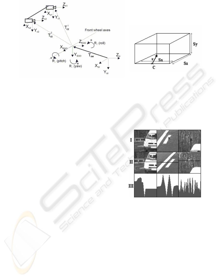
2 ENVIRONMENT MODEL

All 3D entities (points, objects) are expressed in the

world coordinates system, which is depicted in

figure 1.a. This coordinates system, has its origin on

the ground in front of the car, the X axis is always

perpendicular on the driving heading direction, the

Y axes is perpendicular on the road surface and the

Z axis coincides with the driving heading direction.

The ego-car coordinates system has its origin in the

middle of the car front axis, and the tree coordinates

are parallel with the tree main axes of the car. The

world coordinates system is moving along with the

car and thus only a longitudinal and a vertical offset

between the origins of the two coordinates system

exists (vector T

from Figure 1). The relative

orientation of the two coordinates systems (R

rotation matrix) will change due to static and

dynamic factors. The loading of the car is a static

factor. Acceleration, deceleration and steering are

dynamic factors, which also cause the car to change

pitch and roll angles with respect to the road surface.

To obtain the pitch and roll angles and the car height

we measure the distance between the car’s chassis

and wheels because the wheels are on the road

surface. Four sensors are mounted between the

chassis and wheels arms and the car height (T

) and

the pitch(R

) and roll (R

) angles are computed.

Figure 1.a shows also the position of the left and

the right cameras in the ego-car coordinate system.

The position is completely determined by the

translation vectors T

and the rotation matrices

. These parameters are essential for the stereo

reconstruction process and for the epipolar line

computation procedure. In order to estimate them an

offline camera calibration procedure is performed

after the cameras are mounted and fixed on the car

using a general-purpose calibration technique. Due

to the rigid mounting of the stereo system inside the

car these parameters are considered to be

unchangeable during driving.

The stereo reconstruction is performed in the car

coordinates system. The coordinates XX

=[X

, Y

]

of the reconstructed 3D points in the ego-car

coordinates system can be expressed in the world

coordinate system as XX

=[X

, Y

, Z

]

using

the following updating equation:

)(

EWEW

TXXRXX +⋅=

(1)

where T

and R

are the instantaneous relative

position and orientations of the two coordinates

system and are computed from the damper height

sensors by adding an offset to the initial value

(established during camera calibration). The

transformation between the rotation vector and its

corresponding rotation matrix is given by the

Rodrigues (Trucco, 1998) formulas.

)(

],0,[

],,0[

EWEW

ZXEWEWEWEW

YEWEWEWEW

Rodrigues

const

RRrrrr

TTTTT

+=+=

δδδ

δδ

(2)

The objects are represented as cuboids, having a

position (in the world coordinate system), size,

orientation and velocity, as in figure 1.b. The

position (X, Y, Z) and velocity (v

and v

) are

expressed for the central lower point C of the object.

ICINCO 2004 - ROBOTICS AND AUTOMATION

a. b.

Figure 1: a. The world, car and cameras reference systems; b. The object parameters

3 STEREO RECONSTRUCTION

The stereo reconstruction algorithm that is used is

mainly based on the classical stereovision principles

available in the existing literature (Trucco, 1998):

find pairs of left-right correspondent points and map

them into the 3D world using the stereo system

geometry determined by calibration.

Constraints, concerning real-time response of the

system and high confidence of the reconstructed

points, must be used. In order to reduce the search

space and to emphasize the structure of the objects,

only edge points of the left image are correlated to

the right image points. Due to the cameras horizontal

disparity, a gradient-based vertical edge detector was

implemented. Non-maxima suppression and

hysteresis edge linking are being used. By focusing

to the image edges, not only the response time is

improved, but also the correlation task is easier,

since these points are placed in non-uniform image

areas.

Area based correlation is used. For each left edge

point, the right image correspondent is searched. The

sum of absolute differences (SAD) function

(Williamson, 1998) is used as a measure of

similarity, applied on a local neighborhood (5x5 or

7x7 pixels). Parallel processing features of the

processor are used to implement this function. The

search is performed along the epipolar line

computed from the stereo geometry for general

camera configuration.

To have a low rate of false pairs, only strong

responses of the correlation function are considered

as correspondents. If the global minimum of the

function is not strong enough relative to other local

minimums than the current left image point is not

correlated. In figure 2 a successful correlation is

shown along the first column, while the last two

columns show ambiguous similarity functions with

rejected correspondents. Repetitive patterns are

rejected and only robust pairs are reconstructed.

Figure 2: Three correlation scenarios are shown on each

column. Left image point marked by ‘x’ on row I, right

image search area and the epipolar line on row II and the

correlation function on row III.

A parabola is fitted to a local neighborhood (3 or

5 points) of the global correlation minimum in order

to detect the stereo correspondence with sub-pixel

accuracy. The obtained accuracy is about 1/4 to 1/6

and is dependent of the image quality (especially

noise level and contrast). Our tests proved that the 3-

neighbors parabola works better than the other one.

After this step of finding correspondences, each

left-right pair of points is mapped into a unique 3D

point. Two 3D projection rays are traced, using the

camera geometry, one for each point of the pair. By

computing the intersection of the two projection

rays, the coordinates of the 3D point are determined.

STEREOVISION APPROACH FOR OBSTACLE DETECTION ON NON-PLANAR ROADS

4 VERTICAL ROAD PROFILE

ESTIMATION

Many of the obstacle detection methods assume a

flat road profile. Some take into account the car

pitching – therefore admitting some degree of

vertical profile change – but fail to account for a

possible curved vertical profile. We’ll try to extract

the vertical profile of the road by approximating it

with a first order clothoid curve (in the ego-car

coordinate system):

vEE

cZY ++−=

(3)

where:

, is the pitch angle of the ego-car

0,y

– vertical curvature

1,y

– variation of the vertical curvature

In order to extract the coefficients α, c

0,v

and c

1,v

which will completely describe the vertical profile of

the road, we’ll make use of the 3D road points

reconstructed by stereovision. The main advantage

of using stereovision is the ability of directly

extracting the vertical profile, independently of the

lane detection process, sometimes even

independently of the presence of any kind of

delimiters. The key assumption, which makes this

possible, is that there are none or very few 3D points

under the road plane. Having a list of 3D points, it is

easy to obtain a lateral projection in the YOZ plane,

like in figure 3.

As easily can be seen, there is a lot of noise in

the set of points, and therefore a simple fitting of the

curve to the lower points, or a least-square clothoid

fitting is not enough. Our approach to detecting the

vertical profile takes two simplifying assumptions:

- In the close vicinity of the ego-vehicle (20m), the

points are on a straight line, and the effect of the

curvature is sensed only after the 20m interval

- The effect of roll is negligible for the vertical

profile detection, that is, the vertical

displacement due to roll is negligible in

comparison to the displacement due to pitch and

vertical curvature.

These assumptions allow us to regard the

problem as a 2D curve fitting to a set of 2D points

corresponding to the lateral projection of the

reconstructed 3D points (figure 3).

With these assumptions, first we want to estimate

the pitch angle of the ego car coordinate system

relative to the road surface (angle α from equation

3). The pitch angle is extracted using a method

similar to the Hough transform applied on the lateral

projection of the 3D points in the near range of 0-20

m (in which we consider the road flat). Therefore, an

angle histogram is built for each possible pitch

angle, using the near points, and then the histogram

is searched from under the road upwards. The first

angle having a considerable amount of points

aligned to it is taken as the pitch angle.

After detecting the pitch angle, detection of the

curvature follows the same pattern. The pitch angle

is considered known, and then a curvature histogram

is built, for each possible curvature, but this time

only the more distant 3D points (> 20 m) are taken

into account, because the effect of a curvature is felt

only in more distant points. The obtained vertical

clothoid profile of the road is shown in figure 4.

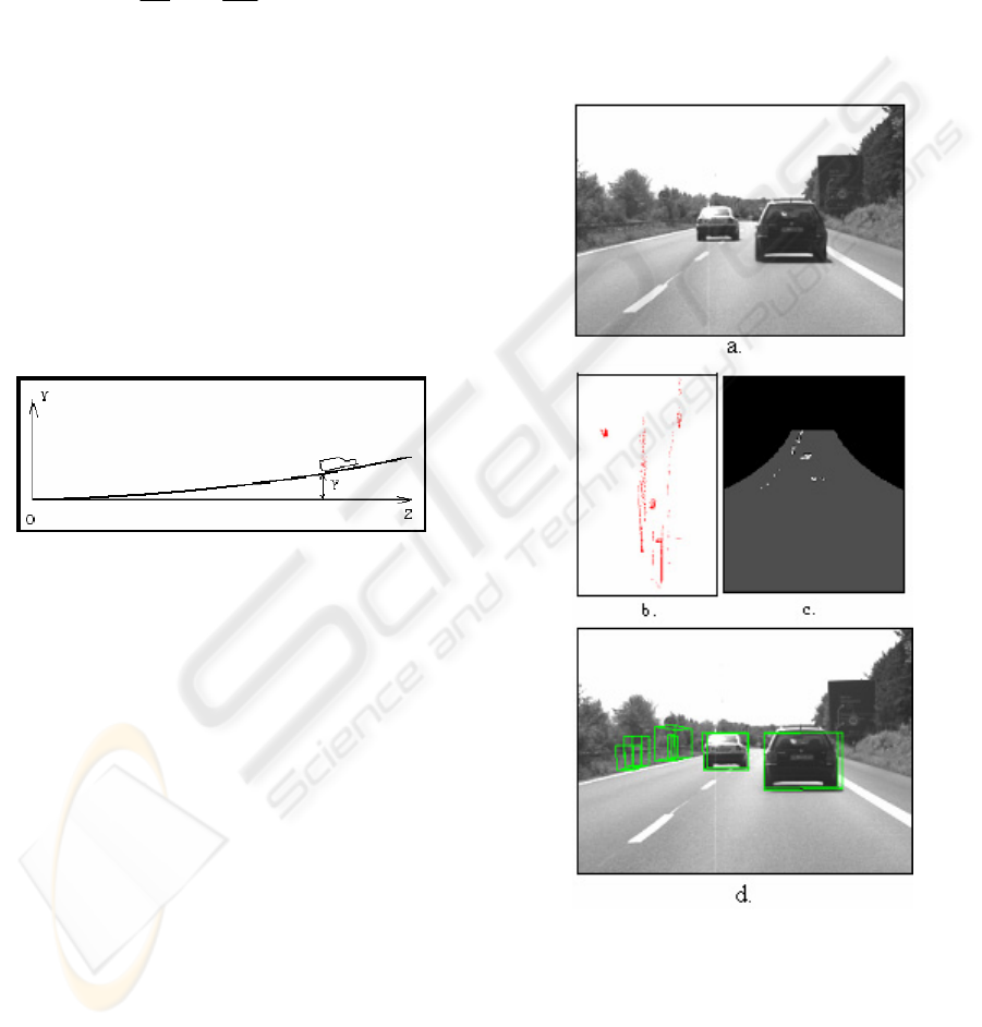
Figure 3: The 3D points in a lateral projection (YOZ plane)

Figure 4: The vertical profile fitted to the ground points

ICINCO 2004 - ROBOTICS AND AUTOMATION

5 GROUPING 3D POINTS INTO

OBJECTS

We use only 3D points situated above the road

surface. The road surface is modeled by the

following clothoid equation in the world coordinates

system:

(4)

The road/obstacle separation (figure 5) of the 3D

points is done using thee following constraints:

− if |Y

-Y| <

, the point is on the road

surface, and classified as road point

− if (Y

-Y) < -

, the point is below the road,

and is rejected

− if (Y

-Y) >

, the point is above the road

The threshold

is a positive constant and its

value is chosen depending on the on the error

estimation of the disparity with the depth, and on the

error estimation of the clothoid parameters and

possible torsion of the road.

Figure 5: Lateral view of the road surface in the world

coordinate system

Some supplementary constraints are used to

restrict the 3D points above the road: points higher

then 4m above the road surface, points that are too

lateral or too far are rejected. The remaining points

belong to the so-called Space of Interest (SOI) in

which is performed the grouping of the 3D points in

objects. For the road geometry we have made the

following assumptions: in highway and most of

country road scenarios the horizontal curvature is

slowly changing and the torsions can be neglected in

our detection range (up to 100m). Therefore

knowing the road vertical profile would be enough

to characterize the driving surface in the SOI.

In our SOI, no object is placed above other. Thus,

on a satellite view of the 3D points in SOI, we are

able to distinguish regions with high points density,

representing and locating objects. Regions with low

density are assumed to contain noisy points and are

neglected. The satellite view (figure 6.b) of the 3D

points detected from the scene depicted in figure 6.a

is analyzed to identify objects.

An important observation is that the 3D points are

more and more rare as the distance grows. To

overcome this phenomenon, we compress the

satellite view of the space (Nedevschi, 2004),

depending on distance, in such a way that local

density of points, in the new space, is kept constant

(figure 6.c. Regardless the distance to an object, in

the compressed space, the region where that object is

located will have the same points density. The

objects are identified as dense regions (figure 6.c).

In figure 6.d the cuboids circumscribing objects are

shown.

Figure 6: a. Reconstructed scene; b. Satellite view of

points. c. The compressed space and the identified objects;

d. Perspective view of object cuboids painted over the

image

STEREOVISION APPROACH FOR OBSTACLE DETECTION ON NON-PLANAR ROADS

6 OBJECT TRACKING

Object tracking is used in order to obtain more stable

results, and also to estimate the velocity of an object

along the axes X and Z. The Y coordinate is tracked

separately, using a simplified approach of simply

averaging the current coordinate by the last detected

coordinate.

The mathematical support of object tracking is

the linear Kalman filter. The position of the object is

considered to be in a uniform motion, with constant

velocity. The position and speed parameters of the

object along the axes X, Y and Z at the moment k

are components of the state vector X(k) that we try

to evaluate through the tracking process. The actual

detection of the object will form the measurement

vector Y(k), which consists only of the coordinates

of the detected object.

[]

zYx

kvkvkvkzkykxk )()()()()()()( =X

(5)

The evolution of the X vector is expressed by the

linear equation:

)1()()( −

= kkk XAX

(6)

where the state transition matrix A(k) is

⎥

⎦

⎤

⎢

⎣

⎡

∆

100000

010000

001000

00100

00010

00001

(7)

The steps of tracking a single object are:

Prediction: a new position of the object is computed

using the last state vector and the transition matrix,

through equation (6).

Measurement: around the predicted position (pX

,pY, pZ) we search for objects resulted from

grouping which have the distance to the

prediction below a threshold. The distance is

computed by equation (8), which gives different

weights to displacements along the three

coordinate axes, and take into consideration also

the current object speed, which is seen as an

indetermination factor.

5.0

7.0

2),,(

pZz

pYy

pXxzyxD

−−+

−+−−=

(8)

The objects that satisfy the vicinity condition

are used to form an envelope whose position is

computed and used as measurement, and the

size of the envelope is used as the current

measurement of the tracked object’s size. By

creating an envelope object out of the objects

near a track we can join objects that were

previously detected as separate. This merging

becomes effective only if the separated objects

have the same trajectory. This is ensured by the

object-track association, when track compete

for objects, and a false object joining won’t last

for too long.

Update: The measurement and the prediction are

used to update the state vector X through the

equations of the Kalman filter. The Y coordinate

and the object’s size are tracked by averaging the

current measurement with the past

measurements. If in the current frame there is no

measurement that can be associated to the track,

the prediction is used as output of the tracking

system. The track is considered lost after a

number of frames without measurement.

Tracking multiple objects adds a little bit more

complexity to the algorithm presented above. We

have to decide which detected object belongs to

which track, or if a detected object starts a new

track. The association between detected objects and

tracks is done using a modified nearest-neighbor

method, using the distance expressed by equation

(8). Each object is compared against each track. The

objects are labeled employing the nearest track

identity number, provided that there is at least one

track that has a sufficient low distance to the object.

The modification from the classical nearest-neighbor

scheme is that we introduce an “age discount” in the

distance comparison, and in this way we give

priority to the older, more established tracks. This

discounting mechanism is achieved by sorting the

tracks in the reverse order of their age (the older

ones first). If we compare an object to a track and

the object already was labeled with the label of

another track, we change the owner of the object

only if the distance object-current track is lower than

the distance to the older track minus a fixed

quantity, the age discount.

For every object that cannot be assigned to an

existing track and that fulfills some specific

conditions, a new track is initialized. A new track is

ICINCO 2004 - ROBOTICS AND AUTOMATION

started for a single object that has a reasonable size.

There is no object joining in the initialization phase

of a track. In this way we avoid initializing tracks to

noise objects, and thus amplifying the noise. Tracks

are aborted if the association process fails for a

predefined number of frames. A tracking validation

process based on the image of the object is

employed in order to ensure that there is no track

switching from one object to another.

7 RESULTS

The detection system has been deployed on a

standard 1 GHz Pentium® III personal computer,

and the whole processing cycle takes less than 100

ms processing time, therefore securing a 10 fps

detection rate. This makes the system suitable for

real-time applications. The system has been tested in

various traffic scenarios, both offline (using stored

sequences) and online (on-board processing), and

acted well in both conditions. In all situations the

obstacles were reliably detected and tracked, and

their position, size and velocity measured. The

detection has proven to have a maximum working

range of about 90 m, with maximum of reliability in

the range 10-60 m. The depth measurement error is,

naturally, higher than one can obtain from a radar

system, but it is very low for a vision system: less

than 10 cm of error at 10 m, about 30 cm of error at

45 m and about 2 m of error at 95 m.

In figure 7 the detection results on a non-flat

road are outlined. The scene from figure 6.a is at the

end of a concave slope. The detected road surface

has a concave vertical curvature

0,v

≈ 2e

-4

. The far

objects (the two cars at 71m, respectively 81m and

the traffic sign from 91m have vertical offsets in the

world coordinates system (having the XOZ plane

coincident with the road surface below the current

car position) of 0.51m, 0.66m and 0.96m

respectively, due to the non flat road. But using the

non-flat road modeled by a vertical clothoid (figure

6.b) the objects are detected correctly on the road

surface.

8 CONCLUSIONS

We have presented a stereovision-based obstacle

detection system that reconstructs and works on 3D

points corresponding to the object edges, in a large

variety of traffic scenarios, and under real-time

constraints. Because the stereovision module

reconstructs any feature in sight (that means also the

road features) the vertical profile of the road was

detected. This way a correct road-obstacle separation

was possible. The grouping of the 3D points in

relevant objects was greatly improved, and the

objects 3D positioning accuracy was increased.

The functions of this system can be greatly

extended in the future. An intelligent correlation

function should be developed, one that can

disambiguate, not reject, repetitive patterns and

reconstruct points from horizontal edges. Moreover,

because any type of object is detected this algorithm

can form the basis for any type of specific object

detection system, such as vehicle detection,

pedestrian detection, or even traffic sign detection.

The classification routines can be performed directly

on our detected objects, with the advantage of

reduced search space and additional helpful

information such as distance, size and speed, which

can also reduce the class hypotheses. The vertical

road profile detection from stereovision can be the

base for a 3D lane detection algorithm, which will

give a complete 3D description of the driving

environment in a lane related coordinates system.

STEREOVISION APPROACH FOR OBSTACLE DETECTION ON NON-PLANAR ROADS

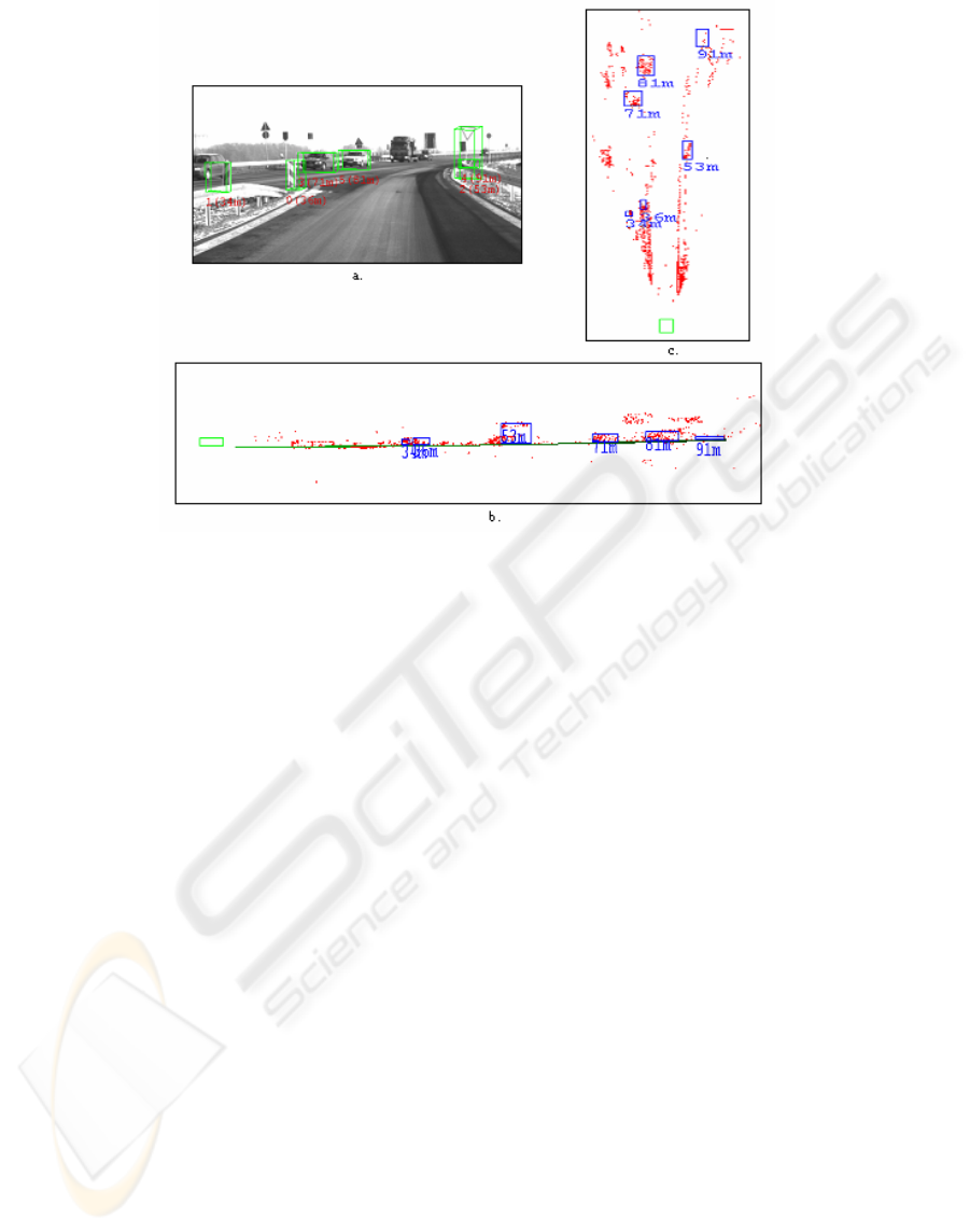
Figure 7: a. Image of the scene with the detected object (cuboids with ID and distance); b. Side view of the detected objects

and the detected road surface; c. Top view of the detected objects.

REFERENCES

Gavrila, D. M, 2000. Pedestrian Detection from a Moving

Vehicle. In Proc. of European Conference on

Computer Vision, Dublin, Ireland, 2000, pp. 37-49

Ulrich, I, Nourbakhsh, I, 2000. Appearance-Based

Obstacle Detection with Monocular Color Vision. In

Proc. of the AAAI National Conference on Artificial

Intelligence, Austin, TX.

Kalinke, T, Tzomakas, C, von Seelen, W, 1998. A Texture

based Object Detection and an Adaptive Model-based

Classification. In Procs. IEEE Intelligent Vehicles

Symposium‘98, (Stuttgart, Germany), pp. 341–346.

Kuehnle, A, 1998. Symmetry-based vehicle location for

AHS. In Procs. SPIE Transportation Sensors and

Controls: Collision Avoidance, Traffic Management,

and ITS, vol. 2902, (Orlando, FL), pp. 19–27.

Nedevschi, S, Schmidt, R., Graf, T, Danescu, R, Frentiu,

D, Marita, T, Oniga, F, Pocol, C, 2004. High Accuracy

Stereo Vision System for Far Distance Obstacle

Detection. In IEEE Intelligent Vehicles Symposium

‘04, Parma, Italy.

Weber, J, Koller, T, Luong, Q.-T, Malik, J, 1995. An

integrated stereo-based approach to automatic vehicle

guidance. In Fifth International Conference on

Computer Vision, In Collision Avoidance and

Automated Traffic Management Sensors, Proc. SPIE

2592.

Williamson, T. A, 1998. A high-performance stereo vision

system for obstacle detection. PhD Thesis CMU-RI-

TR-98-24, Robotics Institute Carnegie Mellon

University, Pittsburg, September.

Hancock, J, 1997. High-Speed Obstacle Detection for

Automated Highway Applications. Tech. Report

CMU-RI-TR-97-17, Robotics Institute, Carnegie

Mellon University, Pittsburg.

Labayrade, R, Aubert, D, Tarel, J P, 2002. Real Time

Obstacle Detection in Stereovision on Non Flat Road

Geometry Through V-disparity Representation. In

Proceedings of IEEE Intelligent Vehicle Symposium,

IV ’02), Versailles, France.

Goldbeck, J, Huertgen, B, 1999. Lane Detection and

Tracking by Video Sensors. In IEEE International

Conference on Intelligent Transportation Systems

(ITSC 99).

Aufrere, R, Chapuis, R, Chausse, F, 2001. A model-driven

approach for real-time road recognition. In Machine

Vision and Applications, Springer-Verlag.

Aufrere, R, Chapuis, R, Chausse, F, 2000. A fast and

robust vision-based road following algorithm. In

IEEE-Intelligent Vehicles Symposium 2000, pp.192-

197.

Takahashi, A, Ninomiya, Y, 1996. Model-based lane

recognition. In Proceedings of the IEEE Intelligent

Vehicles Symposium 1996, pp. 201–206.

Trucco, E, Verri, A, 1998. Introductory Techniques for 3D

Computer Vision. Prentice-Hall, New Jersey.

ICINCO 2004 - ROBOTICS AND AUTOMATION