A FUZZY INTEGRATED APPROACH TO IMPEDANCE CONTROL

OF ROBOT MANIPULATORS

S.J.C. Marques

Polytechnic Institute of Lisbon, Instituto Superior de Engenharia de Lisboa

Department of Mechanical Engineering, Avenida Conselheiro Em

ıdio Navarro, 1900 Lisboa, Portugal

L.F. Baptista, J.M.G. S

a da Costa

Technical University of Lisbon, Instituto Superior T

ecnico

Department of Mechanical Engineering, GCAR/IDMEC, Avenida Rovisco Pais, 1049-001 Lisboa Codex, Portugal

Keywords:

Fuzzy adaptive control, fuzzy sliding mode control, force control, robot manipulators.

Abstract:

This paper presents an integrated fuzzy approach to recover the performance in impedance control, reducing

the errors in position and force, considering uncertainties in the parameters of the manipulator model and

contact surface model. This integrated strategy considers a fuzzy adaptive compensator in the outer control

loop that adjusts the manipulator tip position to compensate for uncertainties present in the environment. In the

inner loop, a fuzzy sliding mode-based impedance controller compensates for uncertainties in the manipulator

model, based on an inverse dynamics control law. The system error, deﬁnes the sliding surfaces of the fuzzy

sliding controller as the difference between the desired and the actual impedances. In order to evaluate the

force/position tracking performance and to validate the proposed control structure, simulations results are

presented with a three-degree-of freedom (3-DOF) PUMA robot.

1 INTRODUCTION

The development of robot manipulator applications

in industry to tasks that involve interaction between

the en-effector and the environment, requires the de-

velopment of more sophisticated force control strate-

gies. Classical force control schemes like hybrid

control (Mason, 1981) or impedance control (Hogan,

1985) are the theoretically foundation of force con-

trol strategies. However, they are not sufﬁcient to

bring robots executing tasks with interaction with a

contact surface, like grinding, deburring and polish-

ing. This lack in performance is due to variable pay-

loads, torque disturbances, parameter variations, un-

modeled robot dynamics and uncertainties in the envi-

ronment parameters. Several approaches to deal with

those uncertainties have been proposed, like classi-

cal adaptive control (Colbaugh et al., 1993), robust

control (Liu and Goldenberg, 1991) and fuzzy adap-

tive control (Hsu and Fu, 1996), among others. A

great research activity in force control has been regis-

tered in the last decade, however, only a few of these

schemes have been implemented in experimental or

industrial robots (Hsu and Fu, 2000; Baptista et al.,

2001). Therefore, more sophisticated control struc-

tures are required to cope with the overall uncertain-

ties in the force control problem.

In this paper, an integrated approach of fuzzy ro-

bust impedance and adaptive control is proposed. In

this approach, an implicit force control formulation is

used to compensate for uncertainties in the manipula-

tor parameters and the contact surface model. The

fuzzy adaptive controller corrects the reference po-

sition to a fuzzy robust impedance controller in the

inner control loop. This controller includes a fuzzy

sliding mode term, where a new sliding surface is de-

ﬁned, based on the impedance error. In the proposed

approach, the impedance controller design is equiva-

lent to the sliding mode controller design.

The outline of the paper is as follows: section 2

presents a brief description of the manipulator dy-

namics in the constrained coordinate frame. Section 3

presents the overall force control structure and a brief

description of the two control schemes. Simulation

results are presented in Section 4, and ﬁnally in Sec-

tion 5 some conclusions are drawn.

2 ROBOT DYNAMICS AND

ENVIRONMENT

Let’s consider an n−link rigid-joint robot manip-

ulator constrained by contact with the environment.

201

Marques S., Baptista L. and Sá da Costa J. (2004).

A FUZZY INTEGRATED APPROACH TO IMPEDANCE CONTROL OF ROBOT MANIPULATORS.

In Proceedings of the First International Conference on Informatics in Control, Automation and Robotics, pages 201-206

DOI: 10.5220/0001139902010206

 SciTePress

The complete dynamic model in cartesian space is de-

scribed by:

(x)¨x + h

(x, ˙x)=u − f

(1)

The vectors x, u and f

∈

(n×1) represent the

end-effector position in the suitable reference coor-

dinate frame, the force control signal, and the force

exerted by the manipulator on the environment, re-

spectively. The term h

is given by C

(x, ˙x) ˙x +

(x)+d

( ˙x), where C

(x, ˙x), g

(x) and d

( ˙x)

are the Coriolis matrix, gravity and friction vectors,

respectively. Generally, a task frame attached to the

constrained surface is selected, when the robot ma-

nipulator tip moves in a force control task, so as to

easily describe the desired position x

and force f

trajectories. The internal joint coordinates q, ˙q and ¨q

must be transformed in external cartesian ones x, ˙x

and ¨x, by means of the forward kinematics, where x

is the position of the tip manipulator in the task frame

coordinates. Regarding the external forces, let’s de-

compose the force vector f

, given by the force sen-

sor in all of its components and already transformed

in the task frame: a normal component f

in the per-

pendicular direction to the surface environment and

a tangential component f

, in the velocity tip manip-

ulator direction. Let’s also assume that the friction

coefﬁcient µ between the manipulator tip and the en-

vironment is known. Thus, it is possible to calcu-

late exactly the perpendicular direction



n to the envi-

ronment surface, implicitly given by the force sensor.

Thus, without lost of generality, only three elements

in force and position, f

and x, deﬁned in its com-

ponents as f

=[f

, 0]

and x =[x

]

respectively, are going to be considered. The force

control is exerted along the ﬁrst component and the

position control is done on the other two components.

In what concerns the environment characteristics, sev-

eral models have been proposed, based on elementary

mechanic components (spring, dump and mass), with

one or two degree of freedom (Epping and Seering,

1987). In this article, the environment is modelled as

a spring mechanical element with stiffness coefﬁcient

3 THE OVERALL CONTROL

STRUCTURE

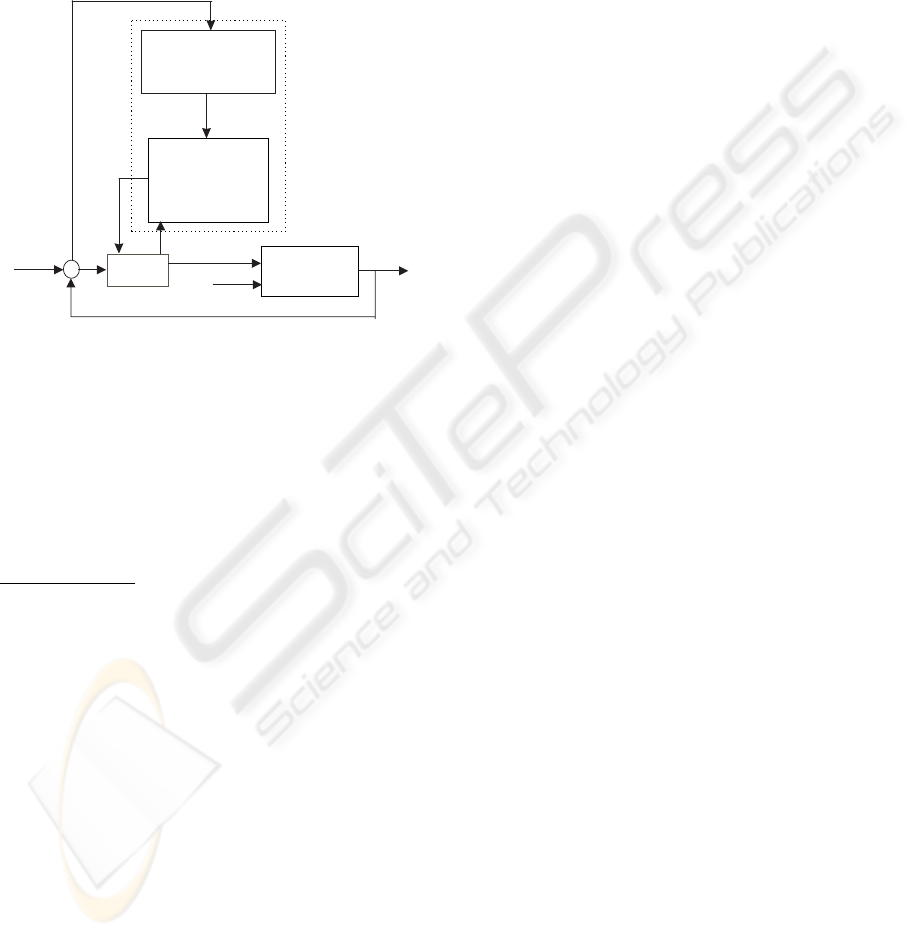
The proposed control structure can be deﬁned as

a position based explicit force control, such that in

the inner loop a position based controller is feeded, in

part, with position errors by a controller in the exter-

nal loop (Fig. 1).

In the external loop, the controller is of fuzzy adap-

tive type, which transforms the force error in a po-

sition adjustment. The main objective of the fuzzy

Fuzzy

Adaptive

Controller

Fuzzy Sliding

Mode-Based

Impedance

Controller

Robot

Figure 1: Block diagram of the overall control structure.

adaptive controller is to compensate environment un-

certainties, like stiffness and geometric location. As

referred above, the fuzzy adaptive controller feeds in

part the inner position controller, because it corrects

only the manipulator tip position x

in the perpen-

dicular direction to the contact surface, based on the

force error e

. Moreover, the inner position controller

will compensate for uncertainties in the manipulator

dynamic model. The inner position controller, is a

fuzzy sliding mode-based impedance algorithm, with

an inverse dynamics control law. As the dynamic

model of the manipulator is not exactly known, an

impedance error will appear. This impedance error

deﬁnes a sliding surface, which, when the system is

in sliding mode, after it has reached the surface, the

state trajectory continues to be on it.

3.1 Fuzzy sliding mode-based

impedance controller

Let’s consider the following impedance control law:

σ = M

(¨x

− ¨x)+B

( ˙x

− ˙x)+

− x) − f

, (2)

where M

, B

and K

are the inertial, damping and

stiffness positive deﬁnite matrices, respectively, and

is the desired position. The second term in (2) van-

ishes when no uncertainties are present in the manip-

ulator dynamic model. When uncertainties are con-

sidered, the second member in (2) assumes a value

with some norm different from zero. As σ = 0 does

not represent a manifold in the state space (x, ˙x), in-

tegrating σ a sliding surface s = 0, can be deﬁned as

(Lu and Goldenberg, 1995):

s = ˙x − ˙x

+ M

−1

(x − x

)+M

−1



dτ

−1



(x − x

)dτ (3)

When the system is in sliding mode, after it has

reached the surface, the state trajectory continues to

be on the sliding surface (s = 0) so that (

s = 0)

and σ = −M

s = 0 is obtained. This indicates that

ICINCO 2004 - ROBOTICS AND AUTOMATION

202

the impedance controller design is equivalent to de-

sign a sliding mode controller which guarantees that

the state trajectory reaches the sliding surface and re-

mains on it, thereafter. The norm of σ is used to repre-

sent the deviation of the system state from the sliding

surface. This deviation reﬂects the impedance control

error.

Let’s consider also an inverse dynamics control law,

based on the robot nominal dynamics:

u =



(x)¨x



(x, ˙x, ˙x

)+f

− K

, (4)

where



(x, ˙x, ˙x



(x, ˙x) ˙x



(x)+



( ˙x) (5)

The velocity ˙x

in (4) and (5), is deﬁned as:

˙x

= ˙x

− M

−1

(x − x

) − M

−1



dτ

−M

−1



(x − x

)dτ (6)

From (3) and (6) the relation ˙x

= ˙x−s holds, which

means that when the state trajectory is on the sliding

surface, the actual velocity ˙x follows ˙x

exactly. The

term K

is given by:

= K

× u

, (7)

where K

is a diagonal matrix of control gains based

on the upper bounds of the uncertainties in the dy-

namic model and u

is a fuzzy system (Lu and

Goldenberg, 1995). This fuzzy system is a counter-

part of the Sliding Mode Controller with Boundary

Layer (SMC-BL). In the boundary layer (BL), near

the sliding line s =0, the control input dynamics

is smoothed, avoiding the chattering effects, ensur-

ing that the error states remain within the layer. In-

side this BL, a null control signal along the switching

line is veriﬁed, and increases the absolute value of the

control signal, as the error states are far away from the

switching line. A fuzzy system with a diagonal form

rule base considering the error and its derivative as in-

puts, has a similar behavior to the above prescribed in

(Palm et al., 1997). However, this rule base can be

reformulated as one input one output, with the input

variable s inside the BL and the output variable u,

accordingly Table 1 and regarding the following rule:

: IF



s is Negative High

THEN



u must be Negative High

This rule base reduces the number of fuzzy rule con-

trol and can assume a more general behavior than the

SMC-BL. In the SMC-BL with boundary layer thick-

ness φ, the control signal u is basically given by:

u = k × sat(

) (8)

Table 1: Reformulated rule base of a fuzzy slid-

ing mode controller with input



s and output



u. (P-

Positive, N-Negative, ZE-Zero, L-Low, M-Medium

and H-High)



s NH NM NL ZE PL PM PH



u NH NM NL ZE PL PM PH

−1 −0.5−0.2 0 0.2 0.5 1

0.5

Input MFs

−1−0.8−0.5 0 0.5 0.8 1

0.5

Output MFs

−1 −0.5 −0.2 0 0.2 0.5 1

−1

−0.8

−0.5

0.5

0.8

Fuzzy System Output

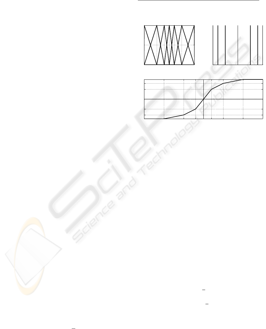
Figure 2: Input and output membership functions and out-

put of the fuzzy system.

This control assumes a linear transfer characteristic

inside the BL. In the FSMC reformulated in that way,

using for instance triangular membership functions

with fuzzy partition leads to stretching the centers

of the input variable towards the origin and expand-

ing the centers of the output variable towards the ex-

tremes. The resulting output of the fuzzy system is

a transfer characteristic with different slopes, which

is greater then 1 near the origin and decreases to-

wards the extremes, where it is less than 1. This is

shown in Fig. 2, where the input and output are nor-

malized into the interval [−1, 1] and different φ

such

that



= φ, that deﬁnes the tracking quality. The

resulting transfer characteristic achieved by this way

must be chosen if for small errors the system is sup-

posed to be more sensitive to disturbances and fast

responses where the error states are near the origin.

As the input of the reformulated FSMC is the variable

s, inside the BL with thickness φ, this can be imple-

mented with the input sat(

), which results in the

normalized interval [−1, 1] by self. This is the same

as the input variable s with

as the scaling factor

of the input variable considering the same normalized

interval. The output of the fuzzy system is inside the

interval [−1, 1], which will be scaled by the elements

of the matrix K

given in (7).

A FUZZY INTEGRATED APPROACH TO IMPEDANCE CONTROL OF ROBOT MANIPULATORS

203

3.2 Fuzzy adaptive controller

The overall fuzzy adaptive control scheme (FAC) pre-

sented in this paper, based on the Fuzzy Model Refer-

ence Learning Controller (Layne and Passino, 1996),

is shown in Fig. 3.

Fuzzy Inverse

Model

Knowledge

Base

Modifier

FLC

Robot +

Controller

Learning

Mechanism

Figure 3: Fuzzy adaptive control scheme (FAC).

The FAC is mainly based on the Fuzzy Logic Con-

troller (FLC), and the learning mechanism. The FLC

is adapted in the membership functions of its conse-

quents by the learning mechanism. The FLC inputs

are the force error e

(kT)=f

(kT) − f

(kT) and

its ﬁnite difference ∆

(kT)=e

(kT)−e

(kT −T )

or the trapezoidal area of the force error δe

(kT)=

(kT )+e

(kT −T )

T . The learning mechanism is com-

posed by the fuzzy inverse model and the knowledge-

base modiﬁer. The fuzzy inverse model attempts to

characterize approximately the representation of the

inverse dynamics of the environment. This is called

by fuzzy inverse model that maps the error in the out-

put variables and possibly other parameters such as

the functions of the error and the process operating

conditions, to the necessary changes in the input pro-

cess (Layne and Passino, 1996). The fuzzy inverse

model is designed to adjust the manipulator tip po-

sition in the perpendicular direction to the environ-

ment surface to compel the force f

(kT) exerted on

it, to be as close as possible to f

(kT). The knowl-

edge base modiﬁer performs the function of modi-

fying the fuzzy controller, in order to improve the

robot’s performance. Based on the necessary changes

given by the output of the fuzzy inverse model p(kT),

the knowledge base modiﬁer changes the member-

ship functions of the FLC consequents, only for those

whose activation level δ

are greater than zero at the

instant (kT − T ). All others remain unchanged. This

can be formulated as:

(kT)=C

(kT − T )+p(kT)

if δ

(kT − T ) > 0; (9)

and

(kT)=C

(kT − T )

if δ

(kT − T )=0 (10)

As shown in (Layne and Passino, 1996), the FAC out-

put that would have been desired, is expressed by:

∆x

∗

(kT − T )=∆x(kT − T )+p(kT) (11)

In the inner position control loop, the FSMC fol-

lows the reference or commanded positions and ve-

locities, given by the path planning algorithm in the

position controlled directions. In the force controlled

direction, those commanded position and velocity are

given by the FAC algorithm. In the last controlled

direction, representing the position and velocity as a

two component vector x

=[x

˙x

]

, the element x

is given by:

= x + u

FAC

, (12)

where x is the actual tip position manipulator and

FAC

is the FAC output. In order to compute the slid-

ing variable along this direction, the vector [e

˙e

]

is given by:

˙e

]

= x − x

= −[u

FAC

˙u

FAC

]

(13)

4 SIMULATION RESULTS

The overall force/position control structure de-

scribed in Section 3 is now applied, by simulation,

to a 3-DOF PUMA 560 robot model, that executes a

trajectory along a ﬂat surface, as shown in Figure 4.

To simulate uncertainties in the environment geome-

try, a mismatch of about 15

◦

between the planned and

the actual plane is imposed. The simulation environ-

ment incorporates the model of the robot, as described

in (Corke, 1996), including the nonlinear arm dynam-

ics and joint friction, providing the basis for a real-

istic evaluation of the controller performance. The

control scheme applied to the robot dynamic model

used in this study, was implemented in the MAT-

LAB/SIMULINK environment, using the Runge-

Kutta fourth order integration method. The control

laws applied to the manipulator model where imple-

mented with a sampling frequency of 1 kHz. The in-

verse dynamics control law of the manipulator only

consider the diagonal terms of the inertial matrix and

the gravitational terms, as shown in Eq. (14):











1,1



2,2



3,3







g



(14)

ICINCO 2004 - ROBOTICS AND AUTOMATION

204

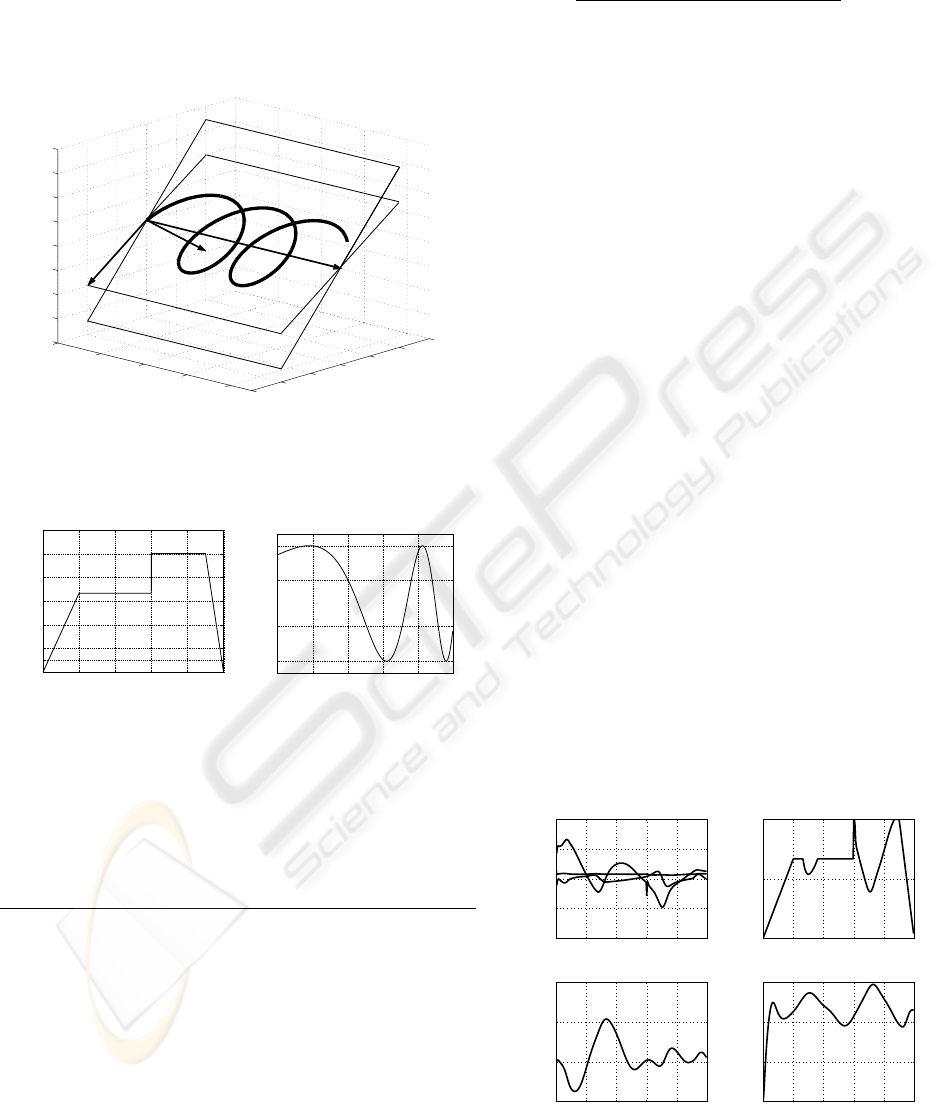
For robustness analysis, the inertial parameters, like

link masses and moments of inertia are disturbed be-

tween 10% and 30% from its nominal value. The de-

sired force path is represented in Fig. 5(a) and the

stiffness coefﬁcient of the environment varies along

time, accordingly Fig. 5(b).

0.1

0.2

0.3

0.4

0.5

0.6

−0.2

0.2

0.4

0.6

−0.1

0.1

0.2

0.3

0.4

0.5

0.6

0.7

Figure 4: Trajectory of the 3-DOF PUMA manipulator.

0 1 2 3 4 5

Force profile

(a)

0 1 2 3 4 5

0.75

0.9

1.1

1.25

x 10

N/m

(b)

Figure 5: a) Desired force proﬁle. b) Environment stiffness.

Table 2: Rule base of the fuzzy inverse model.

e



∆e

NH NM NL Z PL PM PH

PH Z Z PL PL PM PH PH

PM NL Z PL PL PM PM PH

PL NM NL Z PL PL PH PH

Z NH NM NL Z PL PM PH

NL NH NM NL NL Z PL PM

NM NH NM NM NL NL Z PL

NH NH NH NM NL NL Z Z

It is assumed that the manipulator is already in

contact with the surface and the end-effector al-

ways maintains contact with the environment dur-

ing the execution of the task. The impedance

matrices have the following values: M

Table 3: Rule base of the FLC.

e



∆e

NZP

P C

Z C

N C

diag(5, 5, 5), B

= diag(316, 141, 141) and

= diag(5000, 1000, 1000). The boundary

layer thickness for the three subsystems at the

fuzzy sliding mode controller was setting as Φ =

diag(0.05, 0.05, 0.05) and the matrix K

in (7) is

= diag(50, 20, 20) for the three orthogonal di-

rections. Also, the transfer characteristic inside the

boundary layer as presented in Fig. 2 is used, which

reveal an increasing velocity response. The rule base

of the fuzzy inverse model is presented on Table 2 and

the rule base of the FLC has nine rules, accordingly

to Table 3. The centers C

are adapted by the learn-

ing mechanism. It is also assumed that the inputs to

the fuzzy inverse model and to the FLC algorithm are

the same: the force error e

and its difference ∆e

The scaling factors to the fuzzy inverse model are

[8 6; 0.25] and [6 6; 0.0005] for the FLC. All the fuzzy

systems are Takagi-Sugeno type (Palm et al., 1997),

with a fuzzy partition at the antecedents, trapezoidal

shape and singletons C

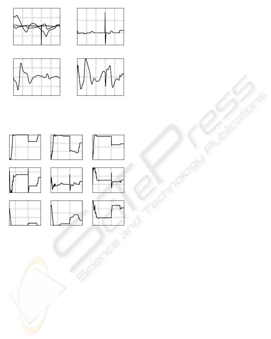
at the consequents. The sim-

ulation results can be observed in Figs. 6, 7 and 8. In

Fig. 6 joint torques, tip position and force errors are

presented without compensation. It can be observed

that the performance is greatly reduced. In Fig. 7 both

fuzzy adaptive and fuzzy sliding controllers compen-

sate for the uncertainties, recovering the performance

of the impedance control. In Fig. 8 the adjustment ac-

tivity of the FLC consequents, done by the learning

mechanism in order to compensate for uncertainties

in the environment, is shown.

0 1 2 3 4 5

−0.01

0.01

0.02

error pos. acc. y

0 1 2 3 4 5

force error

0 1 2 3 4 5

−40

−20

Torque

N.m

0 1 2 3 4 5

0.01

0.02

0.03

error pos. acc. z

Figure 6: Simulation results without compensation.

A FUZZY INTEGRATED APPROACH TO IMPEDANCE CONTROL OF ROBOT MANIPULATORS

205

0 1 2 3 4 5

−2

−1

x 10

−3

error pos. acc. y

0 1 2 3 4 5

−2

force error

0 1 2 3 4 5

−40

−20

Torque

N.m

0 1 2 3 4 5

−5

x 10

−4

error pos. acc. z

Figure 7: Simulation results with compensation of

uncertainties in environment and robot dynamic model.

1 3 5

−1

1 3 5

−0.5

0.5

1 3 5

0.5

1 3 5

−1

−0.5

1 3 5

−0.5

0.5

1 3 5

0.4

0.6

0.8

1 3 5

−1

−0.5

0.5

1 3 5

−1

1 3 5

0.4

0.6

0.8

Figure 8: The adaptation of the consequents of the FLC

membership functions.

5 CONCLUSIONS

In this article, an integration of fuzzy adaptive and

fuzzy robust force/position control to compensate for

overall uncertainties, considering an impedance con-

trol formulation, is presented. The tip position ad-

justed by the fuzzy adaptive controller in the perpen-

dicular direction to the surface, to compensate for un-

certainties in the environment is feeded to an inner

position controller. This controller is a fuzzy slid-

ing mode-based impedance control that compensate

for uncertainties in the manipulator dynamic model.

The adjustment in position done by the fuzzy adap-

tive controller, based on the force error and the ef-

fort done by the fuzzy sliding mode-based impedance

controller in the inner loop, recovers the impedance

control performance and reduces the errors in position

and force. This control structure also exhibits a good

performance considering nonrigid materials with un-

certainties.

Future work will concentrate on the implementation

of this control structure on a industrial PUMA 562

robot.

ACKNOWLEDGEMENTS

This research was partially supported by program

POCTI, FCT, Minist

erio da Ci

encia e do Ensino Su-

perior, Portugal

REFERENCES

Baptista, L., Sousa, J., and S

a da Costa, J. G. (2001). Fuzzy

predictive algorithms applied to real-time force con-

trol. Control Engineering Practice, 9(4):411–423.

Colbaugh, R., Seraji, H., and Glass, K. (1993). Direct adap-

tive impedance control of robot manipulators. Journal

of Robotic Systems, 10:217–242.

Corke, P. (1996). A robotics toolbox for MATLAB. IEEE

Robotics and Automation Magazine, 3(1):24–32.

Epping, S. D. and Seering, W. P. (1987). Introduction to

dynamic models for robot force control. IEEE Control

Systems Magazine, pages 48–51.

Hogan, N. (1985). Impedance control: an approach to ma-

nipulation: Part I-II-III. Journal of Dynamic Systems,

Measurement, and Control, 107:1–24.

Hsu, F.-Y. and Fu, L.-C. (1996). Adaptive fuzzy hybrid

force/position control for robot manipulators follow-

ing contours of an uncertain object. Proc. IEEE Inter-

national Conference on Robotics and Automation.

Hsu, F.-Y. and Fu, L.-C. (2000). Intelligent robot debur-

ring using adaptive fuzzy hybrid position/force con-

trol. IEEE Transactions on Robotics and Automation,

16(4):325–335.

Layne, J. and Passino, K. M. (1996). Fuzzy model reference

learning control. Journal of Intelligent and Fuzzy Sys-

tems, 4:33–47.

Liu, G. J. and Goldenberg, A. A. (1991). Robust hybrid

impedance control of robot manipulators. Proc. IEEE

International Conference on Robotics and Automa-

tion.

Lu, Z. and Goldenberg, A. A. (1995). Robust impedance

control and force regulation: Theory and experi-

ments. International Journal of Robotics Research,

14-3:225–254.

Mason, M. (1981). Compliance and force control for com-

puter controlled manipulators. IEEE Transactions on

Systems, Man and Cybernetics, 11(6):418–432.

Palm, R., Driankov, D., and Hans, H. (1997). Model Based

Fuzzy Control. Springer-Verlag, Berlin Heidellberg.

ICINCO 2004 - ROBOTICS AND AUTOMATION

206