
ROBUST SENSOR BASED NAVIGATION FOR AUTONOMOUS
MOBILE ROBOT
Immanuel Ashokaraj, Antonios Tsourdos, Peter Silson and Brian White
DAPS Department, RMCS, Cranfield University,
Shrivenham, Swindon, UK - SN6 8LA
Keywords:
Interval analysis, Robotics, Navigation.
Abstract:
This paper describes a new approach for mobile robot navigation using an interval analysis based adaptive
mechanism for an Unscented Kalman filter. The robot is equipped with inertial sensors, encoders and ultra-
sonic sensors. The map used for this study is two-dimensional and it is assumed to be known a-priori. Multiple
sensor fusion for robot localisation and navigation has attracted a lot of interest in recent years. An Unscented
Kalman Filter (UKF) is used here to estimate the robots position using the inertial sensors and encoders. Since
the UKF estimates are affected by bias, drift etc, we propose an adaptive mechanism using interval analysis
with ultrasonic sensors to correct these defects in estimates. Interval analysis has been already successfully
used in the past for robot localisation using time of flight sensors. But this IA algorithm has been extended to
incorporate the sensor range limitation as in many real world sensors such as ultrasonic sensors. One of the
problems of the use of interval analysis sensor based navigation and localisation is that it can be applicable
only in the presence of land marks. This problem is overcome here using additional sensors such as encoders
and inertial sensors, which gives an estimate of the robot position using an Unscented Kalman filter in the
absence of land marks. In the presence of land marks the complementary robot position information from the
Interval analysis algorithm using ultrasonic sensors is used to estimate and bound the errors in the UKF robot
position estimate.
1 INTRODUCTION
Robot navigation is primarily about guiding a mobile
robot to a desired destination or along a pre-specified
path in which the robots environment consists of land-
marks and obstacles. In order to achieve this objective
the robot needs to be equipped with sensors suitable
to localize the robot throughout the path it has to fol-
low. Most of these sensors may give overlapping or
complementary information and sometimes be redun-
dant as well. There are many different architectures to
fuse these information. Mobile robots generally carry
dead reckoning sensors such as wheel encoders and
inertial sensors, such as accelerometers, gyroscopes,
to measure acceleration, angle rate and obstacle de-
tecting and map making sensors such as time of flight
ultrasonic sensors. All these sensor measurements
can be fused to estimate the robots position by us-
ing a sensor fusion algorithm. Sensor fusion in this
case is the method of integrating data from distinctly
different sensors to estimate the robots position.
Classical data fusion algorithms use stochastic fil-
ters such as Kalman filters for robot position estima-
tion (Jetto et al., 1999). But one of the main disad-
vantages of using Kalman filters with ultrasonic sen-
sors for robot localisation problems is that the data
association step in Kalman filters is complex and also
the fact that they are often affected by bias and drift.
Moreover an accurate model of the robot system and
accurate statistics of the sensor noises are needed,
which is not available accurately in many cases.
The paper is organised as follows. This introduc-
tory section continues by presenting a background for
the problem of autonomous robot localisation in sec-
tion 1.1, followed by a summary of previous work
in robot localisation using IA and standard stochas-
tic filters in section 1.2. The novelty of the proposed
approach is presented in section 1.3. Section 2 ex-
plains the implementation of the UKF with inertial
sensors and encoders for this problem. Section 3 gives
a brief explanation of the interval analysis algorithm
for robot localisation and also describes how the sen-
sor range limitation is corporated and when multiple
sets of ultrasonic sensor measurements are taken. In
section 4 the implementation of the adaptive mech-
anism for the UKF robot position estimation using
64
Ashokaraj I., Tsourdos A., Silson P. and White B. (2004).
ROBUST SENSOR BASED NAVIGATION FOR AUTONOMOUS MOBILE ROBOT.
In Proceedings of the First International Conference on Informatics in Control, Automation and Robotics, pages 64-70
DOI: 10.5220/0001140500640070
Copyright
c
SciTePress

Interval Analysis with ultrasonic sensors is described
and the results are shown and finally in section 5 the
conclusions are given.
1.1 Background
The problem considered here is that of robot navi-
gation and localisation using multiple low cost sen-
sors such as inertial sensors, encoders and ultra-
sonic sensors. Conventionally stochastic filters such
as Extended Kalman filter or Unscented Kalman fil-
ters (UKF) are used for robot localisation (Clark
et al., 2001). One of the main prerequisites for using
Kalman filter is to have an accurate model of the robot
and also accurate sensor noise statistics (i.e) bias, drift
etc. But in practice it is difficult to have these parame-
ters accurately, especially drift in accelerometers and
gyroscopes, which affects the outcome of the UKF,
there by contributing to errors in the estimated posi-
tion of the robot over a period of time.
Moreover time of flight sensors such as ultrasonic
sensors are used to measure the distance of land marks
from the robot and to recognize the presence of any
obstacles in the robots path. When the 2-D map of
the environment in which the robot travels is known a
priori, the distance measurements from the ultrasonic
sensors can be used independently to estimate the po-
sition of the robot in the map. EKF or UKF can be
used for this purpose as well (Castellanos and Tardos,
1999). But one of the main limitations encountered
when using this approach is the problem of data as-
sociation, as the data association problem in EKF or
UKF is extremely complex and is of the third order
O
3
. There are ways in which this problem can be
simplified to O
2
, but the solution may be suboptimal.
In order to get the best estimate of the robots po-
sition, we can use different types of sensors with dif-
ferent algorithms which have different sources of er-
ror. In this case we use an Unscented Kalman fil-
ter for fusing the data from the accelerometers, gy-
roscopes and encoders and use an Interval Analysis
(IA) algorithm for estimating the robots position us-
ing ultrasonic sensors. IA algorithm is used instead
of EKF or UKF for the ultrasonic sensors because
the IA algorithm can overcome the problems of not
having an accurate model and accurate sensor noise
statistics in the Kalman Filters, as the IA gives a guar-
anteed estimate of the robot position. It should also
be noted that the IA algorithm for ultrasonic sensors
bypasses the complex data association step and han-
dles the problem in a nonlinear way even while been
robust to outliners. Thus we have two independent
sets of the measurements for the robot position. The
estimated robot position using UKF from inertial sen-
sors, which might be affected by bias and drift, are
then fused with the estimated interval robot position
using IA from ultrasonic sensors. The fused robot po-
sition estimate is much better than either one them
alone since the errors in UKF estimated position are
identified and corrected using the IA algorithm.
1.2 Prior work: Robot localisation
with IA using range
measurements
Interval analysis is basically about guaranteed numer-
ical methods for approximating sets. Guaranteed in
this context means that outer (and sometimes inner)
approximations of the sets of interest are obtained,
which can (at least in principle), be made as precise as
desired. Thus interval computation is a special case of
computation on sets, and set theory provides the foun-
dations for interval analysis.
The localisation of an autonomous robot while nav-
igating in a known or partially known environment is
an important problem in mobile robotics. In this sec-
tion an approach for the localisation of the robot us-
ing interval analysis (Kieffer et al., 2000) with sensor
readings from ultrasonic sensors is described briefly.
The main advantage of this method is that it bypasses
the data-association step, which is very complex in
other methods such as Extended Kalman Filters, and
it handles the problem in a nonlinear way without any
linearisation and it is very much robust to outliners.
The robot model described above moves in a
known 2D environment and its motion is planned with
respect to a set of obstacles and landmarks. These
obstacles and landmarks define the world reference
frame W and a robot frame R which is with respect
to the body of the robot.
The robots position is described by the parameters
x
c
, y
c
and θ,which form the configuration vector p =
(x
c
, y
c
, θ)
T
.
So the task now is to estimate the value of the con-
figuration vector p, from a map representing the envi-
ronment of the robot and from distance measurements
provided by a belt of n
s
time of flight sensors with un-
limited range present in the mobile robot. Moreover
since it is assumed that the bounds on the measure-
ment error is known, the resulting distance measure-
ment is in terms of intervals which is stored in an in-
terval vector
[d] = ([d
1
], ...., [d
n
]) (1)
If a model is available to model the ultrasonic sen-
sor interval distance measurements represented by the
interval vector d
m
(p), when the robot configuration
is p, the robot localization problem now becomes a
bounded error parameter estimation problem, namely
that of characterizing the set
P = {p ∈ [p
o
] | d
m
(p) ∈ [d]} (2)
ROBUST SENSOR BASED NAVIGATION FOR AUTONOMOUS MOBILE ROBOT
65

where [p
o
] is an initial search box, assumed to be large
enough to contain all the possible robot configura-
tions. P then contains all the configurations vectors
that are consistent with the given map and measure-
ments.
But the task is to find the configuration vector p and
so the equation given above can be rearranged as
= [p
o
] ∩ (d
m
)
−1
([d]) (3)
(i.e.) for a given configuration vector p the robot eval-
uates the measurements that its sensors would return
and compares then with the actual measurements to
check whether they are consistent.
The problem described by the above mentioned
equation 3 could then be solved using any of the two
approaches namely SIVIA (Set Inversion Via Interval
Analysis) (Jaulin and Walter, 1993) and ImageSP (Ki-
effer et al., 1998). Both the above approaches have
been described in detail in the book by Jaulin et al
(Jaulin et al., 2001) and a brief introduction to both
SIVIA and IMAGESP is given in Sections 3.1, 3.2.
1.3 Novelty
This paper differs for the work in section 1.2 in three
main aspects. Firstly, the above algorithm has been
modified to incorporate sensor range limitation as in
many real world applications. Secondly instead of
using interval values in the kinematic model while
tracking the robot, we use the physical constraints of
the robot model to predict the robot position. Finally
inorder to overcome the scenario when there are no
land marks in the vicinity of the robot, in which case
there will be no measurements from the TOF sensors,
it is proposed to use inertial sensors (INS). Thus in the
presence of land marks, the fusion of the robot posi-
tion from the the INS and TOF sensors is proposed.
2 ROBOT LOCALISATION USING
UKF WITH INERTIAL
SENSORS AND ENCODERS
By fusing the measurement data from the sensors -
wheel encoders, gyroscopes and accelerometers - in
the mobile robot, a reliable estimation of the posi-
tion and heading of the robot can be obtained. There
are basically two well established approaches avail-
able in literature: one is the Kalman filter and the
other is the extended Kalman filter (EKF) (Alessandri
et al., 1997). The Kalman filters are well known meth-
ods used in the theory of stochastic dynamic systems,
which can be used to improve the quality of estimates
of unknown quantities. The difference between the
two methods is that for the first one a linear kinematic
model is used, while for the second one, the EKF a
nonlinear dynamic model is used. We know that, if
we use the nonlinear model, it is much more difficult
to tune the performances of the filter. From the the-
oretical point of view there are no theoretical results
about the convergence properties as well. But in order
to use all the available information, a nonlinear model
is preferred. Most often in real world engineering ap-
plications, the most widespread and reliable state es-
timator for nonlinear systems is the extended Kalman
filter (Sorenson, 1990).
The EKF is the Kalman filter of an approximate
model of the nonlinear system, which is linearised to
the first order around the most recent estimate. As-
suming all the stochastic processes are Gaussian, the
first order linearisation must be carried out at every
iteration before applying the KF algorithms.
For the extended Kalman filter, the robot model
equations can be rewritten as the state equation of the
form shown below,
x
k+1
= f (x
k
, u
k
, w
k
) (4)
which, when linearized will be of the form
x
k+1
≈ ˜x
k+1
+ A(x
k
− ˆx
k
) + Bu
k
+ W w
k−1
, (5)
where, A and B are the jacobian matrix of partial
derivatives.
This first order linearisation using the Taylor series
expansion may introduce errors in the estimated pa-
rameters which may lead to suboptimal performance
and sometimes divergence of the filter.
The above described problem can be overcome to
a certain extent by using a method first described by
Julier and Uhlman as the unscented transform in the
Kalman filter for the linearisation process (Julier and
Uhlmann, 1997). This formulation of the Kalman fil-
ter is called the Unscented Kalman Filter. The un-
scented transform is basically a deterministic sam-
pling approach, where the state distribution is approx-
imated by a gaussian random variable, but is now de-
scribed using a minimal set of carefully chosen sam-
ple points. These sample points are chosen using the
unscented transform method which completely de-
scribes the true mean and covariance of the gaussian
random variable. When these chosen points are prop-
agated through the true non-linear system, it can cap-
ture the posterior mean and covariance accurately up
to the 3rd order for Taylor series expansion, where as
in a EKF we can achieve only up to first-order accu-
racy. It should also be noted that the computational
complexity of the UKF is the same order as that of
EKF. The basic equations for the UKF has been given
in detail in the book (Wan and der Merwe, 2001)
All the process noises are assumed to be zero mean,
uncorrelated white random noises only.
In the measurement model for this robot there are
four sources of observations that are considered:
ICINCO 2004 - ROBOTICS AND AUTOMATION
66
1. velocity measurements from the wheel encoders,
2. acceleration from the accelerometers, which when
integrated gives the velocity of the robot,
3. robot heading angle measurement from the en-
coders and
4. the angular velocity measurements from the rate
gyroscope which when integrated once gives the
heading angle of the robot.
Thus, for both the velocity and heading angle of the
robot there are two sets of measurements from two in-
dependent sensors. These two sets of measurements
are then given as input to the Kalman filter which esti-
mates the robots speed and heading angle, from which
the robots position can then be calculated.
3 ROBOT LOCALISATION WITH
INTERVAL ANALYSIS USING
RANGE MEASUREMENTS
In this section the robot localisation using IA as first
described briefly in section 3 is further improved us-
ing multiple measurements from the ultrasonic sensor
measurements.
A brief overview of the algorithm for a single mea-
surement has been given in the Figures 3, 4 and 5 .
The main improvement in this version of the algo-
rithm in the descriptions in the tables is that the range
of the ultrasonic sensor has been limited to 3 meters,
where as in (Kieffer et al., 2000) the range was unlim-
ited. This is implemented by identifying the sensors
n
i
that only give readings less than 3 meters (which
is done by setting all the interval ranges greater than
3 meters to infinity in Figure 5) and substituting them
for instead of n
s
(where the inclusion function was
calculated for all the n
s
number of sensors) in the
Figure 4. Also it is assumed that the land marks are
spaced sparsely (i.e) there is a distance of at least 3
meters between the landmarks. This is because when
the land marks are close some of the land marks may
not be visible to the robot sensor model in the IA algo-
rithm. Additionally the land marks which are visible
to the robot in the 3 meter radius are only given to the
inclusion function in Figure 4 instead of all the n
w
segments, there by saving computational time.
This problem as given in equation 3 is then solved
using any of the two approaches namely SIVIA (Set
Inversion Via Interval Analysis) (Jaulin and Walter,
1993) and ImageSP. A brief introduction to both
SIVIA and IMAGESP is given in the next two sub-
sections.
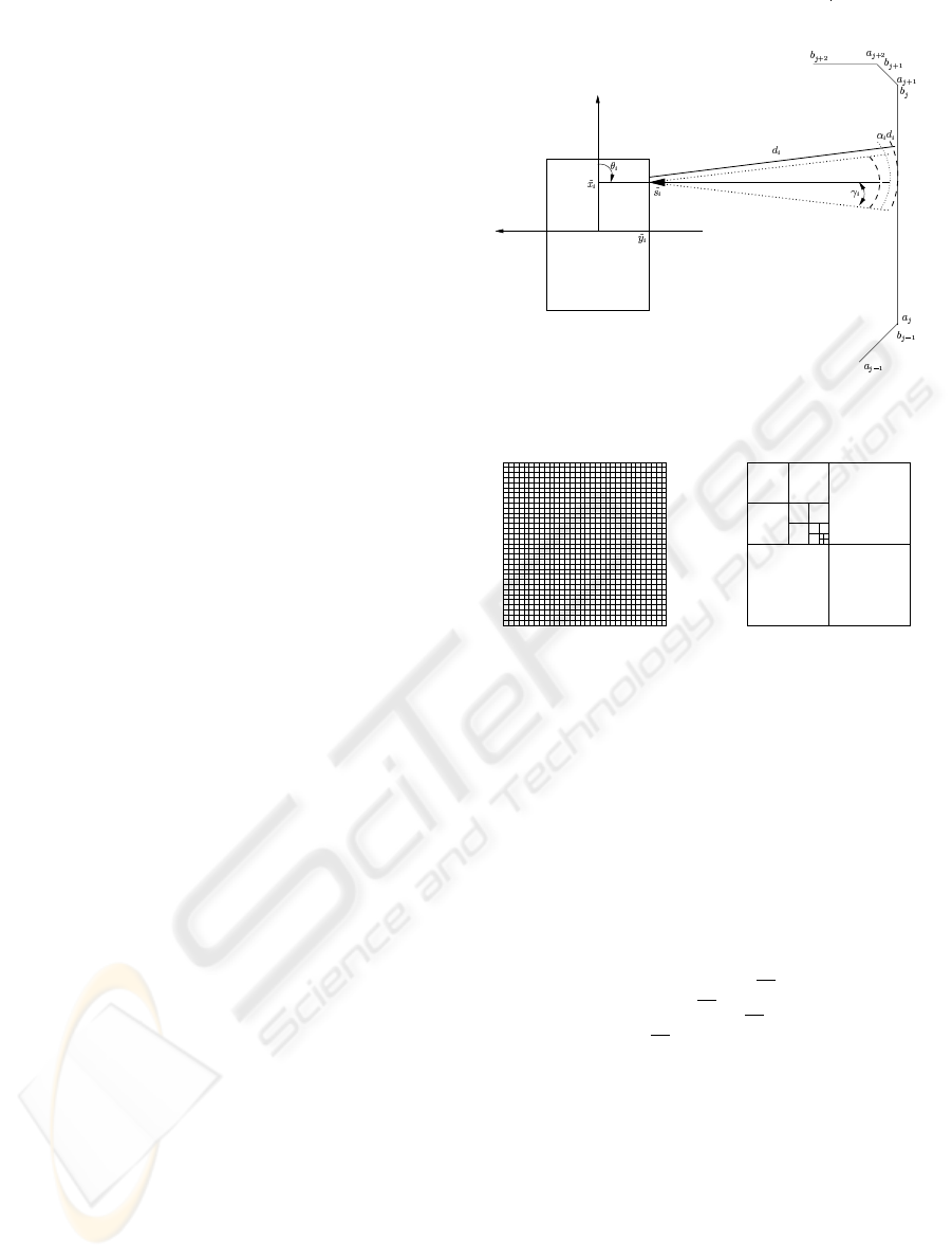
R
Figure 1: Robot and Sensor model
SIVIA AlgorithmImageSp Algorithm
Figure 2: A schematic representation of ImageSp and
SIVIA algorithm
3.1 Set Inversion Via Interval
Analysis (SIVIA)
Set inversion is the computation of the reciprocal im-
age
X = {x ∈ R
n
| f (x) ∈ Y } = f
−1
(Y ) (6)
of a regular subpaving Y of R
m
by a possibly nonlin-
ear function f : R
n
→ R
m
and SIVIA is a method to
compute two subpavings X
and X of R
n
such that
X ⊂ X ⊂ X (7)
A subpaving is a finite set of non-overlapping boxes
that are all included in the same root box. It is called
regular if each of the boxes can be obtained by a finite
succession of bisections and selections (Jaulin et al.,
2001).
In this problem for robot localisation, P = {p ∈
[p
o
] | t(p) = 1}, SIVIA can be applied (Kieffer
et al., 2000). Therefore in this case, if t
[]
([p
o
]) = 1,
p
o
is in the solution set P and is stored in
b
P . If
t
[]
([p
o
]) = 0 then [p
o
] has an empty intersection
with P and is dropped from further consideration. If
t
[]
([p
o
]) = [0, 1] and if the width of [p
o
] is larger
than the pre-specified precision parameter ² , then p
o
is bisected, leading to two child sub boxes L(p) and
ROBUST SENSOR BASED NAVIGATION FOR AUTONOMOUS MOBILE ROBOT
67

Algorithm d
m
(in: p; out: d
m
)
1 for i := 1 to n
s
2 s
i
:=
µ
x
c
y
c
+
µ
cos θ − sin θ
sin θ cos θ
es
i
3
−→
u
1i
:=
Ã
cos(θ +
e
θ
i
− γ)
sin(θ +
e
θ
i
− γ)
!
;
−→
u
2i
:=
Ã
cos(θ +
e
θ
i
+ γ)
sin(θ +
e
θ
i
+ γ)
!
;
4 (d
m
)
i
(p) := +∞;
5 for j := 1 to n
w
(d
m
)
i
(p) :=
min
¡
(d
m
)
i
(p) , r
¡
s
i
,
−→
u
1i
,
−→
u
2i
, a
j
, b
j
¢¢
.
Figure 3: Model for calculating the distance expected from
ultrasonic sensor when the configuration is p
R(p), and the test t
[]
(.) is recursively applied to both
of them. Any box with width smaller than ² is con-
sidered to be small enough and it is added to
b
P . A
diagram explaining SIVIA is given in Figure 2.
3.2 IMAGE SubPaving (IMAGESP)
When f is not invertible, a specific and computation-
ally more demanding procedure is used. The basic
idea of IMAGESP algorithm is to describe the ini-
tial search box p
o
using a subpaving consisting of p
boxes whose width are less than ². Then IMAGESP
evaluates the image of each of these p boxes using an
inclusion function f
[]
of f and stores them on a list.
Therefore we will be getting p image boxes, each of
which contains the true image set of the associated
initial box. At last, IMAGESP merges all these im-
age boxes into a subpaving to allow further processing
(Kieffer et al., 1999). A diagrammatic representation
of IMAGESP is given in Figure 2.
Thus the actual position of the robot represented
here by the configuration vector p at any given instant
of time can be found using SIVIA or IMAGESP algo-
rithms.
The Figure 1 gives a brief description of a map that
represents the surroundings in which the robot travels
(which is assumed to be known in order to calculate
d
m
(p)) and also the measurement process.
A detailed description of the above inclusion func-
tions has been provided by (Kieffer et al., 2000).
Also a better version of the above algorithm in terms
of computational time, incorporating the interval ele-
mentary tests to eliminate some of the infeasible con-
figurations in the configuration vector has been de-
scribed in (Kieffer et al., 2000), in which the problem
is reformulated as P = {p ∈ [p
o
] | t(p) holdstrue}
(i.e.) P = {p ∈ [p
o
] | t(p) = 1} , where t(p) is
a global test. The global test t(p) consists of vari-
ous elementary tests (three tests (Kieffer et al., 2000))
and they are robust to outliners as well. Also the
Algorithm [d
m
] (in: [p;] out: [d
m
])
1 for i := 1 to n
s
2 [s
i
] :=
µ
x
c
y
c
+
µ
cos[θ] − sin[θ]
sin[θ] cos[θ]
es
i
3
−−→
[u
1i
] :=
Ã
cos([θ] +
e
θ
i
− γ)
sin([θ] +
e
θ
i
− γ)
!
;
−−→
[u
2i
] :=
Ã
cos([θ] +
e
θ
i
+ γ)
sin([θ] +
e
θ
i
+ γ)
!
;
4 [d
m
]
i
([p]) := +∞;
5 for j := 1 to n
w
[d
m
]
i
([p]) :=
min
³
[d
m
]
i
([p]) , [r]
³
[s
i
] ,
−−→
[u
1i
],
−−→
[u
2i
], a
j
, b
j
´´
.
Figure 4: Inclusion function for the measurement model
Algorithm [r] (in : [s], [
−→
u
1
], [
−→
u
2
], a, b; out : [r]);
1. [t
r
] :=
³
det
³
−→
ab,
−→
as
´
≥ 0
´
if [t
r
] = 0 then [r] := +∞; return;
2. [t
h
] :=
³D
−→
ab,
−−→
a [s]
E
≥ 0
´
∧
³D
−→
ba,
−→
b[s]
E
≥ 0
´
∧
³D
−→
ab,
−−→
[u
1
]
E
≤ 0
´
∧
³D
−→
ab,
−−→
[u
2
]
E
≥ 0
´
;
3. [r
h
] := [χ] ([t
h
] , [l] ([s] , (a, b)) , +∞) ;
4. [t
a
] :=
³
det
³
−−→
[u
1
],
−−→
[s] a
´
≥ 0
´
∧
³
det
³
−−→
[u
2
],
−−→
[s] a
´
≤ 0
´
;
5. [r
a
] := [χ]
³
[t
a
] ,
°
°
°
−−→
[s] a
°
°
°
, +∞
´
;
6. [t
b
] :=
³
det
³
−−→
[u
1
],
−−→
[s] b
´
≥ 0
´
∧
³
det
³
−−→
[u
2
],
−−→
[s] b
´
≤ 0
´
;
7. [r
b
] := [χ]
³
[t
b
] ,
°
°
°
−−→
[s] b
°
°
°
, +∞
´
;
8. for i := 1 to 2
9.
£
t
h
i
¤
:=
³
det
³
−−→
[s] a,
−→
[u
i
]
´
≥ 0
´
∧
³
det
³
−−→
[s] b,
−→
[u
i
]
´
≤ 0
´
;
10.
£
r
h
i
¤
:= [χ]
³
£
t
h
i
¤
,
h
l
−−→
[u
i
]
i
([s] , (a, b)) , +∞
´
;
11. [r] := min
¡
[r
h
] , [r
a
] , [r
b
] ,
£
r
h
1
¤
,
£
r
h
2
¤¢
;
12. [r] := [χ] ([t
r
] , [r] , +∞) .
Figure 5: Inclusion function for the remoteness of the cone
from a segment
purpose of the first two tests is to eliminate some in-
feasible configurations there by saving computational
time. But if all the three tests are used when the range
of the sensor is limited, it leads to scenarios in which
some feasible configurations are ignored prematurely.
Therefore only two tests were used (inroom test and
the data test in (Kieffer et al., 2000)). The main con-
sequence of not using the leg-in test when the sensor
range is limited is that it may increase the computa-
tion time.
In the case when the robot is moving the robots po-
sition needs to be tracked, in which case the robots
position needs to predicted at the next instant to esti-
mate the robots position at that instant. This is done
by using the physical limitations of the robot based
on the maximum speed and heading angle rate of the
robot, instead of using a kinematic model of the robot.
Thus we obtain an independent position of the robot
from the ultrasonic sensors.
ICINCO 2004 - ROBOTICS AND AUTOMATION
68
forInterval Analysis algorithm
robot position estimation
coordinates
Interval X and Interval Y
robot coordinates which forms
a box or a plane
Inertial Sensors
Ultrasonic
sensors
Map of robot
environment
Sensor fusion block diagram
Encoders
robot speed and orientation
Robot
X and Y coordinate
OR
UKF Sensor fusion for estimating
UKF estimated X and Y robot
Check whether the UKF robot position is inside the interval robot position box.
If so the robot position is the UKF estimated X and Y coordinates.
If not the robot position is the point which is closest to the UKF estimate in the interval box.
Figure 6: Block diagram of IA based adaptive mechanism
for UKF
−10 −5 0 5 10
−10
−5
0
5
10
UKF only estimated robot position
X coordinate (m)
Y coordinate (m)
Land Marks
Actual robot
position
UKF estimated
robot position
Figure 7: UKF only estimated robot position
4 INTERVAL ANALYSIS BASED
ADAPTIVE MECHANISM FOR
UKF
Sensor fusion is a very important and keenly re-
searched topic in the domain of mobile robotics. This
is due to the fact that, instead of using bespoke expen-
sive sensors for estimating the robots position, mul-
tiple low cost sensors can be used, there by reducing
the cost of developing the robot. Moreover these same
sensors can be used to do other tasks other than esti-
mating the robots position such as building the map of
the robots environment using ultrasonic sensors etc.
Also the source of errors in one sensor may be differ-
ent from another one and this fact can be exploited to
eliminate the errors in the measurements.
For the problem of sensor fusion stochastic filters,
such as Kalman filters, are commonly used. But they
suffer from the same disadvantages described before
−10 −5 0 5 10
−10
−5
0
5
10
X coordinate (m)
Y coordinate (m)
UKF estimated robot position with IA based adaptive mechanism using SIVIA algorithm
Land Marks
Actual robot
position
Interval robot
position
IA based adaptive
UKF robot
postion estimate
Figure 8: Fused robot position using SIVIA algorithm as
adaptive mechanism in UKF
(i.e.) an accurate model of the system and statics are
needed. In order to overcome these difficulties while
using the UKF, a new approach has been introduced in
this paper. As described above the robots position are
estimated using two independent sources namely, the
robot position from inertial sensors and the interval
robot position from ultrasonic sensors.
The position obtained using interval analysis is up-
dated only once every second, where as the position
from inertial sensors and encoders are updated 100
times per second as it has a sampling time of 0.01
seconds. Moreover we know that the robots interval
position to be guaranteed (even though in a few cases
it may not be due to the way the boxes are subdivided
but still they are very close to the actual position). The
interval position thus obtained will therefore be like a
plane or rectangle. Then the estimated position using
the inertial sensors is checked whether they are inside
this rectangle. In case they are present inside the rect-
angle then they are trusted to be accurate and used.
Alternatively if they are not then both the measure-
ments are fused by selecting the point on the rectangle
(box) (i.e.) the interval robot position, which is geo-
metrically closest to the robot position estimated us-
ing UKF with inertial sensors, thereby bounding the
error in the UKF estimates. A block diagram of the
sensor fusion method is given in Figure 6.
But since the UKF estimates of inertial sensors is
not accurate as they may be affected by bias, drift etc
and also as the robot is slow moving, instead of using
a dynamic interval model of the robot to predict the
next step as in (Jaulin et al., 2001) we use the physical
limitations of the robot to predict the next step in the
Interval Analysis algorithm.
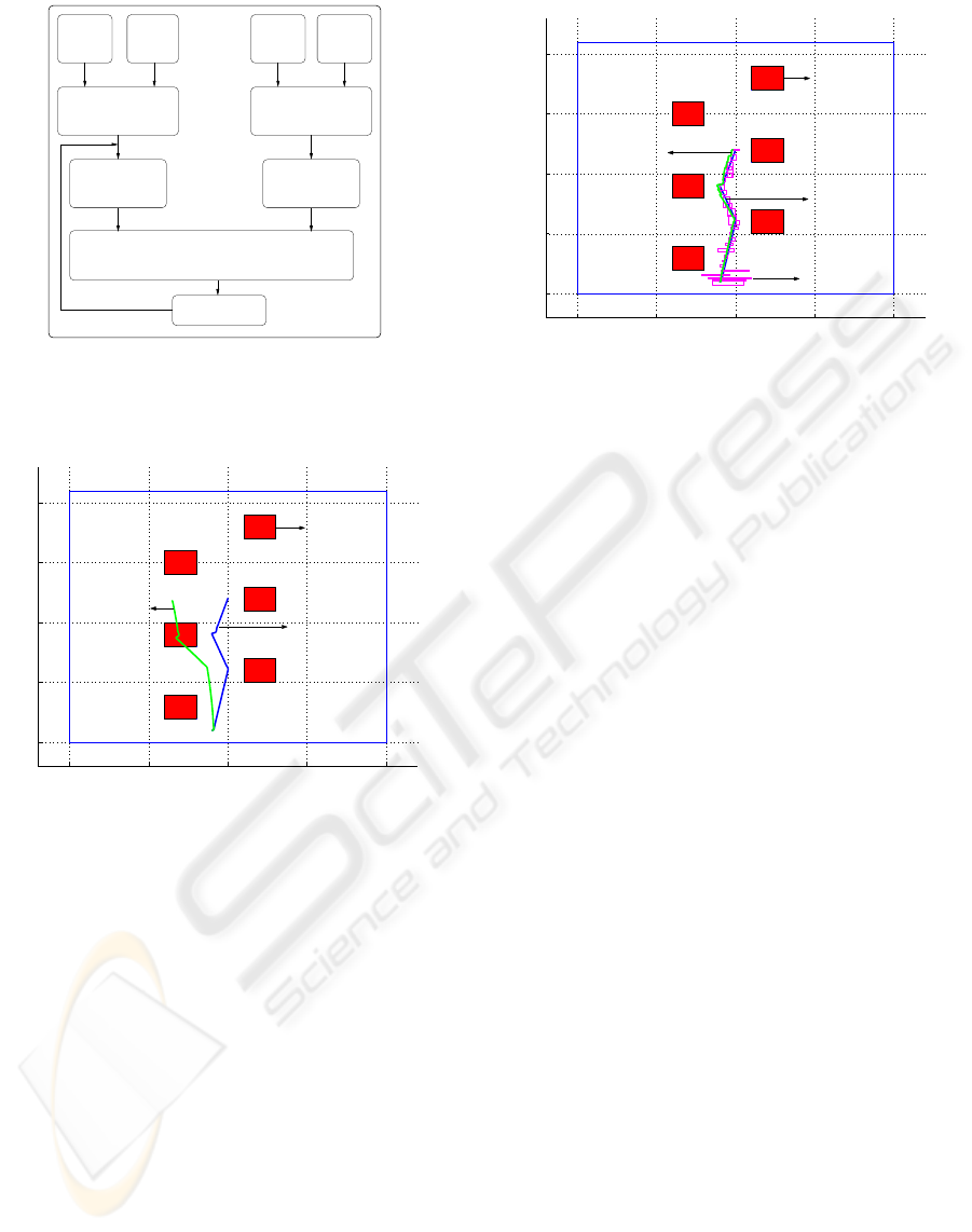
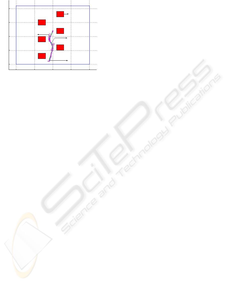
The above described algorithm was successfully
implemented and tested in simulation using MAT-
LAB and C++ software. The Figure 8 shows the robot
position after using the adaptive UKF robot position
ROBUST SENSOR BASED NAVIGATION FOR AUTONOMOUS MOBILE ROBOT
69
−10 −5 0 5 10
−10
−5
0
5
10
UKF estimated robot position with IA based adaptive mechanism using IMAGESP
X coordinate (m)
Y coordinate (m)
Obstacles or
Land Marks
Actual robot
position
Interval robot
position
IA based adaptive
UKF robot position
estimate
Figure 9: Fused robot position using IMAGESP algorithm
as adaptive mechanism in UKF
estimate using the SIVIA interval robot position esti-
mate for adaptation. It can be seen that the interval po-
sition estimate is very conservative when there are no
land marks in one coordinate, for example at the be-
ginning of the robot path in Figure 8. Moreover it can
be observed that the UKF estimate with the interval
analysis based adaptive mechanism has significantly
improved the UKF robot position estimate when com-
pared with the UKF position estimate without the IA
adaptive mechanism shown in Figure 7. Similarly the
Figure 9 shows the UKF robot position estimation us-
ing the IMAGESP algorithm for the adaptive mecha-
nism. It should be noted that the SIVIA interval posi-
tion uncertainty is more when compared with the IM-
AGESP algorithm, but the computational complexity
for the IMAGESP algorithm is more when compared
with the SIVIA algorithm.
5 CONCLUSION
An Unscented Kalman filter (UKF) using an Inter-
val Analysis based adaptive mechanism has been de-
scribed. The UKF uses accelerometers, gyroscopes
and encoders to measure the robots speed and head-
ing angle, so that the robots position can be estimated.
But the UKF robot position estimate is affected by er-
rors in robot model, sensor bias, drift etc. The Interval
Analysis (IA) is a deterministic approach to estimat-
ing the robots position without using a model of the
robot system, thereby minimizing errors due to robot
model. The interval analysis algorithm with ultra-
sonic sensor measurement to estimate robot position
has been described. Additionally previous work on
robot localisation and navigation using interval anal-
ysis has been extended so to incorporate sensor range
limitation. Moreover instead of using dynamic inter-
val model of the robot to predict the next step of the
interval robot position while tracking the robot posi-
tion, the physical limitations of the robot are used to
predict the next step in the interval analysis algorithm.
The IA robot position estimate is then used for an
adaptive mechanism to correct the errors in the UKF
robot position estimate. Then the newly implemented
approach to fuse both these robot position estimation
has been described and it can be observed that the
UKF with the IA based adaptive mechanism gives a
much accurate estimate when compared to estimates
with UKF without the adaptive mechanism.
REFERENCES
Alessandri, A., Bartolini, G., Pavanati, P., Punta, E., and
Vinci, A. (1997). An application of the ekf for inte-
grated navigation in mobile robotics. American Con-
trol Conference.
Castellanos, J. and Tardos, J. (1999). Mobile Robot Lo-
calisation and Map Building: A Multisensor Fusion
Approach. Kluwer Ac. Pub., Boston.
Clark, S., Dissanayake, G., Newman, P., and Durrant-
Whyte, H. (2001). A solution to slam problem. IEEE
Journal of Robotics and Automation, 17(3).
Jaulin, L., Kieffer, M., Didrit, O., and Walter, E. (2001).
Applied Interval Analysis with examples in parame-
ter and state estimation robust control and robotics.
Springer-Verlag, London.
Jaulin, L. and Walter, E. (1993). Set inversion via interval
analysis for nonlinear bounded-error estimation. Au-
tomatica, 29(4):1053 to 1064.
Jetto, L., Longhi, S., and Venturini, G. (1999). Develop-
ment and experimental validation of an adaptive ekf
for the localization of mobile robot. IEEE Transac-
tions on Robotics and Automation, 15(2).
Julier, S. and Uhlmann, J. (1997). A new extension of
the kalman filter to nonlinear systems. In Proc. of
Aerosense: The 11thInt. Symp. on Aerospace/Sensing,
Simulation and Controls.
Kieffer, M., Jaulin, L., Didrit, O., and Walter, E. (2000).
Robust autonomous robot localization using interval
analysis. Reliable Computing, 6(3):337 to 362.
Kieffer, M., Jaulin, L., and Walter, E. (1998). Guaran-
teed recursive nonlinear state estimation using interval
analysis. Internal Report, Laboratoire des Signaux et
Systemes.
Kieffer, M., Jaulin, L., Walter, E., and Meizel, D. (1999).
Guaranteed mobile robot tracking using interval anal-
ysis. Proceedings of the MISC’99 Workshop on Appli-
cations of Interval Analysis to Systems and Control,
page 347 to 359.
Sorenson, H. (1990). Kalman filtering theory and applica-
tion. IEEE press.
Wan, E. and der Merwe, R. V. (2001). Kalman Filtering and
Neural Networks, Chapter 7: The Unscented Kalman
Filter. Wiley Publishing.
ICINCO 2004 - ROBOTICS AND AUTOMATION
70
