
LINEAR MODELLING AND IDENTIFICATION OF A MOBILE
ROBOT WITH DIFFERENTIAL DRIVE
Patr
´
ıcia N. Guerra
∗
Pablo J. Alsina
∗
Adelardo A. D. Medeiros
∗
Ant
ˆ
onio P. Ara
´
ujo
∗
Federal University of Rio Grande do Norte – Departament of Computer Engineering and Automation
UFRN-CT-DCA – Campus Universit
´
ario – 59072-970 Natal RN Brazil
Keywords:
Nonholonomic robots, robot control, stabilization control, linear modeling of robots.
Abstract:
This paper presents a modelling and identification method for a wheeled mobile robot, including the actuator
dynamics. Instead of the classic modelling approach, where the robot position coordinates (x, y) are utilized as
state variables (resulting in a non linear model), the proposed discrete model is based on the travelled distance
increment ∆l. Thus, the resulting model is linear and time invariant and it can be identified through classical
methods such as Recursive Least Mean Squares. This approach has a problem: ∆l can not directly measured.
In this paper, this problem is solved using an estimate
f
∆l based on a second order curve approximation.
Experimental data were colected and the proposed method was used to identify the model of a real robot.
1 INTRODUCTION
Usually, realistic mathematical models of mobile
robots are obtained through the physics laws that gov-
ern their behavior. Approaches applying artificial in-
telligence techniques to the input and output measure-
ments are also utilized. Several model types were de-
veloped for non holonomic mobile robots. LTI (linear
time invariant) models are usually obtained through
Taylor series linearization on only one point of opera-
tion of the system. A QLPV (quasi-linear parameter-
varying) model for a car-like robot is presented in the
literature (Economou et al., 2002).
The classic mathematical model of a mobile robot
has a structure similar to the mathematical model of
robot manipulators, so that techniques of parametric
identification developed for the latter can be adapted
for the former. However, most of these techniques as-
sume that robot speed and acceleration measurements
are available, which is not generally true.
Differently of the identification techniques for ma-
nipulators, enough discussed in the literature (Poignet
and Gautier, 2000; Efe et al., 1999), the mobile
robot identification techniques have been less stud-
ied. An identification of the dynamic model of a
micro-robot using the recursive least mean square
1
The authors received partial financial support of the
Brazilian agencies CAPES and CNPq.
method (RLMS) is presented by Pereira (Pereira,
2000; Pereira et al., 2000). As the model to be iden-
tified through RLMS is non linear, a simplification is
used: the orientation θ(t), which is time-variant, is
considered constant during each sampling period.
In this work a linear (not a linearized one) dynamic
model for mobile robots is presented. The proposed
model is equivalent to the non linear dynamic model,
commonly adopted for non-holonomic mobile robots
(Yamamoto et al., 2003). The proposed model uses
the variable ∆l, distance traveled by the robot during
a sampling interval, instead of the traditional mod-
elling, where its absolute position is used (x, y). The
problem due to the impossibility of measuring the
traveled distance ∆l during a sampling period is over-
come through the use of an estimate,
f
∆l, of this value.
The identification of this discrete dynamic model is
attained using a classic method of identification of lin-
ear systems, the recursive least mean squares.
The rest of this paper is organized as follows. Sec-
tion 2 describes the robot and its modelling by the
equivalent linear and non-linear models. Section 3
presents the proposed calculation method for a nu-
meric value of the immeasurable variable ∆l. In sec-
tion 4, experimental results validating the proposed
approach are shown. Finally, in section 5, the ob-
tained results are discussed and the conclusions and
future perspectives are presented.
263
Guerra P., Alsina P., Medeiros A. and Araújo A. (2004).
LINEAR MODELLING AND IDENTIFICATION OF A MOBILE ROBOT WITH DIFFERENTIAL DRIVE.
In Proceedings of the First International Conference on Informatics in Control, Automation and Robotics, pages 263-269
DOI: 10.5220/0001140602630269
Copyright
c
SciTePress
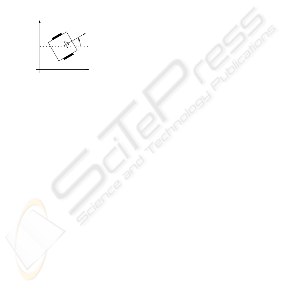
2 ROBOT MODELLING
Figure 1 presents a diagram of the kind of robot we
consider in this work. The robot has two wheels,
driven by two independent electric motors. The
wheels are placed at each side of the robot, in such
a position that their rotation axis are coincident. The
robot configuration is represented by the position of
the center of the axis between the two wheels in the
Cartesian space (x and y) and by its orientation θ (an-
gle between the vector of the robot orientation and the
abscissas axis).
v
x
y
θ,ω
Figure 1: Robot modelling
2.1 Cinematic Model
The cinematic model describes the relations between
the derivatives of robot position and orientation and
the robot linear and angular speeds, v and w, without
taking into account the causes of its movement:
˙x
˙y
˙
θ
=
"
cos θ 0
sin θ 0
0 1
#
·
·
v
w
¸
(1)
This equation models the non-holonomic restrictions
of the robot, due to the fact of its wheels not allowing
lateral movements.
2.2 Dynamic Model
The dynamic model is derived from the physics laws
that govern the several robot subsystems, including
the actuator dynamics (electric and mechanical char-
acteristics of the motors), friction and robot dynamics
(movement equations). The derivation of this model
for a small mobile robot (Vieira et al., 2001) was pre-
sented by Yamamoto (Yamamoto et al., 2003).
For most robots, the modelling process generates a
second-order model expressed by equation 2:
Ku = M
˙
v + Bv (2)
where v = [
v w
]
T
represents the robot linear and
angular speeds, u = [
e
r
e
l
]
T
contains the input
signals (usually armature tensions) applied to the right
and left motors, K is the matrix which transforms the
electrical signals u into forces to be generated by the
robot wheels, M is the generalized inertia matrix and
B is the generalized damping matrix, which includes
terms of viscous friction and electric resistance.
2.3 Equivalent Linear Model
The complete robot model, obtained from the union of
equations 1 and 2, can be represented by the following
state equation:
˙v
˙ω
˙x
˙y
˙
θ
=
−M
−1
B
.
.
. 0
. . . . . . . . . . . . . . .
cos(θ) 0
sin(θ) 0
0 1
.
.
. 0
v
ω
x
y
θ
+
M
−1
K
. . . . . . .
0
·
e
r
e
l
¸
y =
"
0 0 1 0 0
0 0 0 1 0
0 0 0 0 1
#
v
ω
x
y
θ
(3)
where the system output y = [
x y θ
]
T
corre-
sponds to the robot configuration.
To allow the application of linear discretization
techniques, we will rewrite the system equations into
a linear representation of the robot dynamic behav-
ior. To attain this objective, we need to change the set
of state variables: the robot’s configuration, given by
its position x and y and its orientation θ, will be de-
scribed in terms of the robot linear displacement l and
the robot orientation θ.
˙v
˙ω
˙
l
˙
θ
=
−M
−1
B
.
.
. 0
. . . . . . . . . . . . .
1 0
0 1
.
.
. 0
v
ω
l
θ
+
M
−1
K
. . . . . . .
0
·
e
r
e
l
¸
z =
·
0 0 1 0
0 0 0 1
¸
v
ω
l
θ
(4)
The new state equation 4 has the same dynamic
parameters than the original state equation 3 but a
new system output z = [
l θ
]
T
. We observe
that the linear equivalent model was obtained with-
out any simplification assumption. In this way, the
linear model is an exact equivalent representation of
the original non-linear representation in equation 3.
ICINCO 2004 - ROBOTICS AND AUTOMATION
264
2.4 Model Discretization
To allow the application of the classical estimation
techniques, it is necessary to derive a discrete transfer
function equivalent to the model in equation 4. The
first step is the transformation of the state space form
into a continuous transfer matrix:
·
L(s)
θ(s)
¸
=
·
G
11
(s) G
12
(s)
G
21
(s) G
22
(s)
¸
·
·
E
r
(s)
E
l
(s)
¸
(5)
where each term G
ij
(s) has the following structure:
G
ij
(s) =
N
ij
(s)
D(s)
=
α
ij
s + β
ij
s(s
2
+ k
1
s + k
2
)
In the second step, we calculate the four discrete
transfer functions G
ij
(z):
·
L(z)
θ(z)
¸
=
·
G
11
(z) G
12
(z)
G
21
(z) G
22
(z)
¸
·
·
E
r
(z)
E
l
(z)
¸
(6)
where each term G
ij
(z) has the following structure:
G
ij
(z) =
N
ij
(z)
D(z)
=
γ
ij
z
2
+ δ
ij
z + ²
ij
(z − 1)(z
2
+ α
1
z + α
2
)
To obtain a parametrisation appropriated to the pa-
rameter estimation, the transfer functions are con-
verted to equivalent difference equations:
∆l
k
= − α
1
∆l
k−1
− α
2
∆l
k−2
+ (7)
+ γ
11
e
r,k−1
+ δ
11
e
r,k−2
+ ²
11
e
r,k−3
+
+ γ
12
e
l,k−1
+ δ
12
e
l,k−2
+ ²
12
e
l,k−3
∆θ
k
= − α
1
∆θ
k−1
− α
2
∆θ
k−2
+ (8)
+ γ
21
e
r,k−1
+ δ
21
e
r,k−2
+ ²
21
e
r,k−3
+
+ γ
22
e
l,k−1
+ δ
22
e
l,k−2
+ ²
22
e
l,k−3
where ∆l
k
= l
k
− l
k−1
is the linear distance traveled
in a sampling period, ∆θ
k
= θ
k
− θ
k−1
is the an-
gular increment in the robot’s orientation in the same
period, and e
r,k
and e
l,k
are the plant input signals.
3 TRAVELED DISTANCE
COMPUTATION
The variable ∆l is not measurable. In spite of this,
we can use heuristics to calculate a plausible value
for this variable,
f
∆l. The methodology developed to
calculate
f
∆l consists of the following steps:
1. calculation of the path length |
f
∆l|
2. calculation of the direction of the movement, i.e.
the sign of
f
∆l
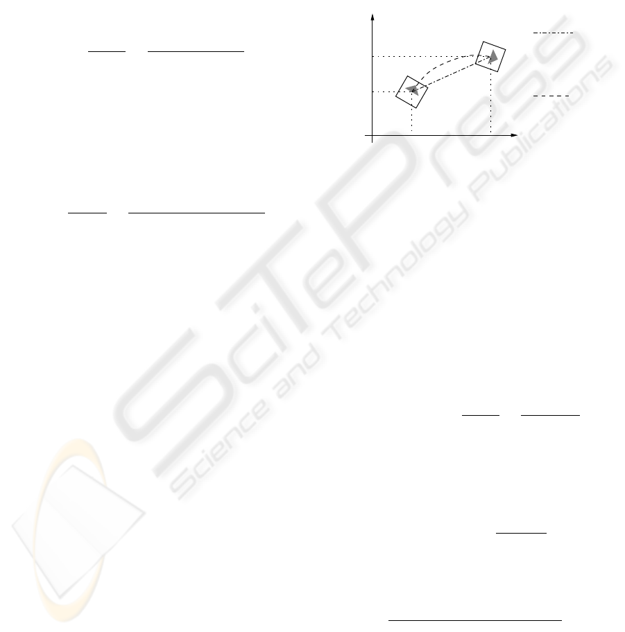
3.1 Path Length Computation
It is possible to obtain with reasonable precision the
robot configuration (x, y, θ) in two consecutive sam-
pling instants, but we cannot be sure about the path
traveled by the robot between the first configuration
and the second configuration. However, a parametric
curve (x(λ), y(λ)), 0 ≤ λ ≤ 1 can be interpolated
between these points and the length of this curve can
be used as an estimated value of |
f
∆l| (see figure 2).
y
0
y
1
x
0
x
1
λ = 0
λ = 1
1
st
degree
polynomial
2
nd
degree
polynomial
Figure 2: Diagram for |
f
∆l| computation
Adopting a 1
st
order polynomial to interpolate, we
are using the Euclidean distance as a measure of the
length of the traveled distance. However, this solution
violates the non-holonomic constraints of the system
when the traveled path is not a straight line.
In this work, we used a parametric curve of 2
nd
degree to calculate the absolute value of
f
∆l because
this is the simplest polynomial allowing interpolating
between the two configurations without violating the
non-holonomics constrains at the contour conditions:
x(λ) = a
2
λ
2
+ a
1
λ + a
0
y(λ) = b
2
λ
2
+ b
1
λ + b
0
tan[θ(λ)] = d(λ) =
dy/dλ
dx/dλ
=
2b
2
λ + b
1
2a
2
λ + a
1
(9)
x(0) = x
0
= a
0
y(0) = y
0
= b
0
x(1) = x
1
= a
2
+ a
1
+ a
0
y(1) = y
1
= b
2
+ b
1
+ b
0
d(0) = tan(θ
0
) = b
1
/a
1
d(1) = tan(θ
1
) =
2b
2
+ b
1
2a
2
+ a
1
(10)
Solving the system 10 results in the following gen-
eral solution:
a
0
= x
0
a
1
=
2[tan(θ
1
)(x
1
− x
0
) − y
1
+ y
0
]
tan(θ
1
) − tan(θ
0
)
a
2
= x
1
− x
0
− a
1
b
0
= y
0
b
1
= a
1
tan(θ
0
)
b
2
= y
1
− y
0
− b
1
(11)
LINEAR MODELLING AND IDENTIFICATION OF A MOBILE ROBOT WITH DIFFERENTIAL DRIVE
265
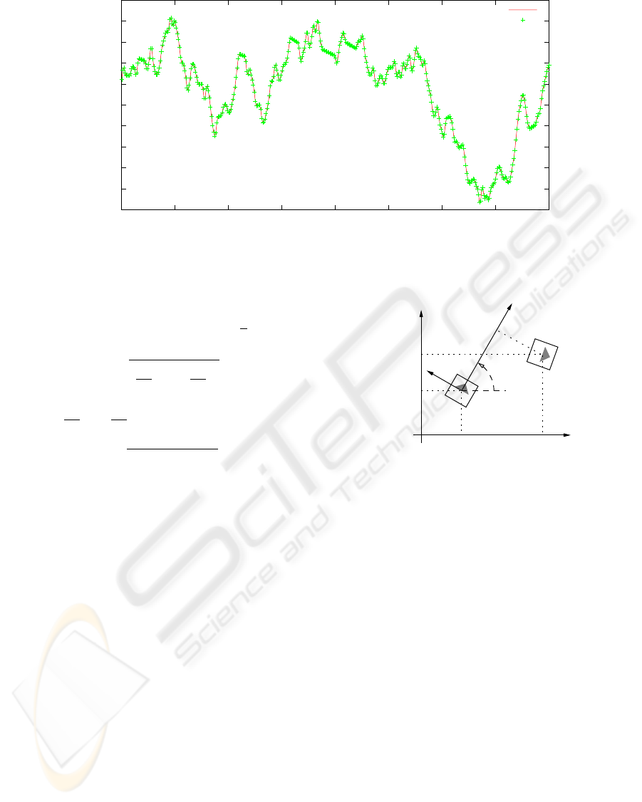
-0.003
-0.0025
-0.002
-0.0015
-0.001
-0.0005
0
0.0005
0.001
0.0015
0.002
0 50 100 150 200 250 300 350 400
delta_L(m)
number of iterations
calculated from non-linear simulation
linear simulation
Figure 3: Comparison between
f
∆l and ∆l
Similar solutions can be found for the singular
cases where θ
0
or θ
1
have values close to ±
π
2
.
To calculate the length of this curve, we used:
g
|∆l| =
Z
1
0
r
(
dx
dλ
)
2
+ (
dy
dλ
)
2
dλ (12)
Substituting
dx
dλ
and
dy
dλ
in equation 12 we obtain:
g
|∆l| =
Z
1
0
p
Aλ
2
+ Bλ + C dλ (13)
where
A = 4a
2
2
+ 4b
2
2
B = 4a
1
a
2
+ 4b
1
b
2
C = a
2
1
+ b
2
1
(14)
The closed solution for the integral in equation 13
can be found in integral tables.
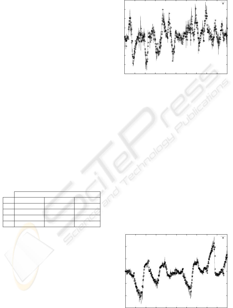
3.2 Computation of the Movement
Direction
To obtain the sign of the traveled distance, i.e. know-
ing if the robot moved forward or backward, we cal-
culate the value of
0
x
1
, the x coordinate of the cur-
rent configuration point (x
1
, y
1
) calculated with re-
spect to the reference frame attached to the previous
robot position (x
0
, y
0
), as indicated in the figure 4.
If
0
x
1
is positive, the robot will have moved forward
and
f
∆l > 0. Otherwise, the robot will have moved
backward and
f
∆l < 0.
A simple coordinate transformation allows the cal-
culation of
0
x
1
:
0
x
1
= x
1
cos θ
0
− x
0
cos θ
0
+
+ y
1
sin θ
0
− y
0
sin θ
0
(15)
y
0
y
1
x
0
x
1
0
x
1
θ
0
Figure 4: Diagram for calculating the sign of
f
∆l
3.3 Validation of Traveled Distance
Computation
Several tests were performed to validate the approxi-
mation of ∆l by
f
∆l. We simulated the linear system
described by equation 4 and the non-linear system de-
scribed by equation 3 with the same input values (e
r
and e
l
), obtaining as outputs, respectively:
z =
·
l
θ
¸
and y =
"
x
y
θ
#
After this, we plotted the values of ∆l = l
k
− l
k−1
,
generated by the linear system, and
f
∆l, which was
calculated using the x and y outputs generated by
the non-linear system and the proposed approxima-
tion. From figure 3, we can observe that
f
∆l (esti-
mated value) is very close to the actual distance trav-
eled by the robot (∆l). The mean error was 0,058%,
with a standard deviation of 0,274%.
ICINCO 2004 - ROBOTICS AND AUTOMATION
266
4 EXPERIMENTAL RESULTS
The results presented in this section were obtained us-
ing a small (7.5 × 7.5 × 7.5cm) mobile robot, with
two wheels driven by two independent DC motors,
very used in robot soccer competitions. A detailed
description of the robot can be found in precedent ar-
ticles (Vieira et al., 2001).
The inputs signals e
r
and e
l
are the armature volt-
ages of the right and left DC motors. The system out-
put y = [
x y θ
]
T
is measured by processing
the image from a fixed camera placed over the robot
workspace (Aires et al., 2001). We use a sampling
rate of 30 samples per second, fixed by the image ac-
quisition card.
The classical method of Recursive Least Mean
Squares (
˚
Astr
¨
om and Wittenmark, 1997) was utilized
for the estimation of the parameters of the model
(equations 7 and 8). The system was excited with
pseudo-random input signals, assuming values be-
tween 1.0 (100% of the motor supply voltage, 9V)
and -1.0 (-9V). As the robot has some high time con-
stants, the input values only changed at each 8 sam-
pling periods. To reduce the chance of high velocities,
the tensions near 0.0 were more probable than the ten-
sions near ±1.0.
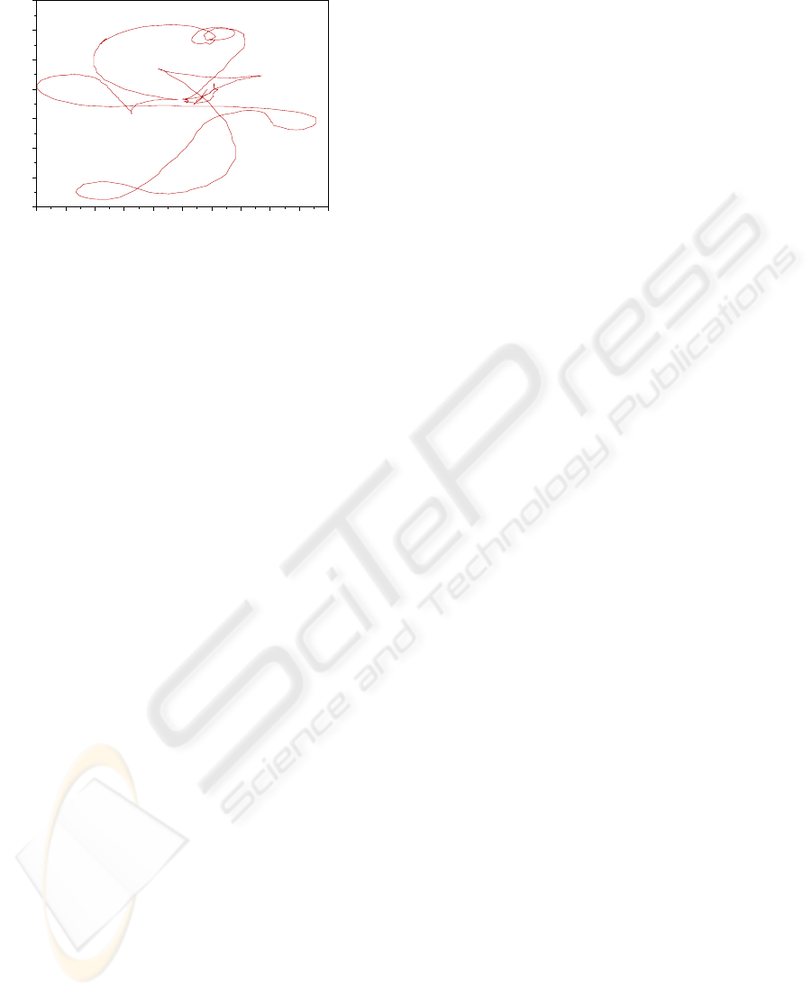
Figure 9 shows the trajectory followed by the robot
during an experiment with 500 samples. The resulting
estimated parameters are presented in table 1.
Table 1: Estimated parameters
α
1
=-0.2125 α
2
=-0.5362
ij γ
ij
δ
ij
²
ij
11 -0.0005195 -0.0005098 0.003019
12 -0.0001753 -0.001158 0.003347
21 0.01099 -0.02627 -0.03326
22 0.001818 -0.06038 0.1074
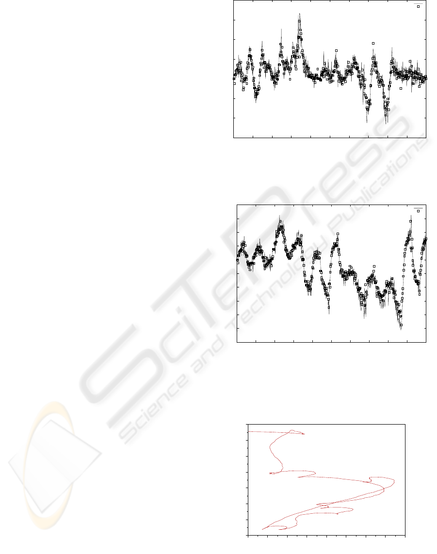
Figure 5 shows the measured and estimated val-
ues for ∆θ. The error in the estimation of ∆θ has
mean value of 0.000426rad and standard deviation of
0.0685rad. Figure 6 shows the calculated values of
f
∆l and the estimated values for ∆l. The error in the
estimation of ∆l has mean value of -0.000297m and
standard deviation of 0.00261m.
To validate the generality of the obtained model,
we calculate the estimation errors using the same pa-
rameters with a different trajectory (figure 10). Figure
7 shows the measured and estimated values for ∆θ
(mean value of 0.00878rad and standard deviation of
0.0814rad) and figure 8 shows the calculated values
of
f
∆l and the estimated values for ∆l (mean value of
-0.000435m and standard deviation of 0.00267m).
-0.4
-0.3
-0.2
-0.1
0
0.1
0.2
0.3
0.4
0 50 100 150 200 250 300 350 400 450 500
measured
estimated
Figure 5: ∆θ measured and ∆θ estimated
5 CONCLUSION
We proposed the substitution of the robot position
variables (x, y) by the distance traveled in a sampling
period ∆l. This substitution resulted in an equivalent
exact linear dynamic model, suitable for identification
through the standard linear systems methods. More-
over, the linearity of the proposed model allows its ap-
plication on the design of dynamic controllers based
on classic linear discrete techniques, as proposed by
Vieira (Vieira et al., 2004).
It can be observed that, in spite of the fact that the
identified model have been defined in the discrete do-
main, there is no impediment of obtaining the contin-
uous model from the same, also allowing its use in the
design of controllers in the continuous domain.
-0.03
-0.02
-0.01
0
0.01
0.02
0.03
0 50 100 150 200 250 300 350 400 450 500
measured(calculated)
estimated
Figure 6:
f
∆l calculated and ∆l estimated
LINEAR MODELLING AND IDENTIFICATION OF A MOBILE ROBOT WITH DIFFERENTIAL DRIVE
267
REFERENCES
Aires, K. R. T., Alsina, P. J., and Medeiros, A. A. D. (2001).
A global vision system for mobile mini-robots. In
SBAI - Simp
´
osio Brasileiro de Automac¸
˜
ao Inteligente,
Canela, RS, Brasil.
˚
Astr
¨
om, K. J. and Wittenmark, B. (1997). Computer Con-
troled Systems. Information and System Sciences.
Prentice-Hall, EUA, 3 edition. ISBN 0-13-314899-8.
Economou, J., Tsourdos, A., and White, B. (2002). Takagi-
sugeno model synthesis of a quasi-linear parameter
varying mobile robot. In IROS - IEEE/RSJ Interna-
tional Conference on Intelligent Robots and Systems,
volume 3, pages 2103–2108.
Efe, M., Kaynak, O., and Rudas, I. (1999). A novel com-
putationally intelligent architecture for identification
and control of nonlinear systems. In ICRA - IEEE In-
ternational Conference on Robotics and Automation,
volume 3, pages 2073–2077, Detroit, MI, USA.
Pereira, G. A. S. (2000). Identificac¸
˜
ao e controle de micro-
rob
ˆ
os m
´
oveis. Master’s thesis, Universidade Federal
de Minas Gerais, Belo Horizonte, MG, Brazil.
Pereira, G. A. S., Campos, M. F. M., and Aguirres, L. A.
(2000). Modelo din
ˆ
amico para predic¸
˜
ao da posic¸
˜
ao
e orientac¸
˜
ao de micro-rob
ˆ
os m
´
oveis observados por
vis
˜
ao computacional. In CBA - Congresso Brasileiro
de Autom
´
atica, Florian
´
opolis, SC, Brazil.
Poignet, P. and Gautier, M. (2000). Comparison of weighted
least squares and extended kalman filtering methods
for dynamic identification of robots. In ICRA - IEEE
International Conference on Robotics and Automa-
tion, volume 4, pages 3622–3627, San Francisco, CA,
USA.
Vieira, F. C., Alsina, P. J., and Medeiros, A. A. D. (2001).
Micro-robot soccer team - mechanical and hardware
implementation. In Congresso Brasileiro de Engen-
haria Mec
ˆ
anica, pages 534–540.
Vieira, F. C., Medeiros, A. A. D., Alsina, P. J., and
Ara
´
ujo Jr., A. P. (2004). Position and orientation con-
trol of a two-wheeled differentially driven nonholo-
nomic mobile robot. In ICINCO – International Con-
ference on Informatics in Control, Automation and
Robotics, Set
´
ubal, Portugal.
Yamamoto, M. M., Pedrosa, D. P. F., and Medeiros, A.
A. D. (2003). Um simulador din
ˆ
amico para mini-
rob
ˆ
os m
´
oveis com modelagem de colises. In SBAI -
Simp
´
osio Brasileiro de Automac¸
˜
ao Inteligente, Bauru,
SP, Brazil.
-0.6
-0.4
-0.2
0
0.2
0.4
0.6
0.8
0 50 100 150 200 250 300 350 400 450 500
measured
estimated
Figure 7: ∆θ measured and ∆θ estimated
-0.03
-0.025
-0.02
-0.015
-0.01
-0.005
0
0.005
0.01
0.015
0.02
0 50 100 150 200 250 300 350 400 450 500
measured(calculated)
estimated
Figure 8:
f
∆l calculated and ∆l estimated
−0.25 −0.21 −0.17 −0.13 −0.09 −0.05 −0.01 0.03 0.07
−0.7
−0.5
−0.3
−0.1
0.1
0.3
0.5
0.7
0
−0.25 −0.21 −0.17 −0.13 −0.09 −0.05 −0.01 0.03 0.07
−0.7
−0.5
−0.3
−0.1
0.1
0.3
0.5
0.7
×
−0.25 −0.21 −0.17 −0.13 −0.09 −0.05 −0.01 0.03 0.07
−0.7
−0.5
−0.3
−0.1
0.1
0.3
0.5
0.7
×
50
−0.25 −0.21 −0.17 −0.13 −0.09 −0.05 −0.01 0.03 0.07
−0.7
−0.5
−0.3
−0.1
0.1
0.3
0.5
0.7
×
100
−0.25 −0.21 −0.17 −0.13 −0.09 −0.05 −0.01 0.03 0.07
−0.7
−0.5
−0.3
−0.1
0.1
0.3
0.5
0.7
×
150
−0.25 −0.21 −0.17 −0.13 −0.09 −0.05 −0.01 0.03 0.07
−0.7
−0.5
−0.3
−0.1
0.1
0.3
0.5
0.7
×
200
−0.25 −0.21 −0.17 −0.13 −0.09 −0.05 −0.01 0.03 0.07
−0.7
−0.5
−0.3
−0.1
0.1
0.3
0.5
0.7
×
250
−0.25 −0.21 −0.17 −0.13 −0.09 −0.05 −0.01 0.03 0.07
−0.7
−0.5
−0.3
−0.1
0.1
0.3
0.5
0.7
×
300
−0.25 −0.21 −0.17 −0.13 −0.09 −0.05 −0.01 0.03 0.07
−0.7
−0.5
−0.3
−0.1
0.1
0.3
0.5
0.7
×
350
−0.25 −0.21 −0.17 −0.13 −0.09 −0.05 −0.01 0.03 0.07
−0.7
−0.5
−0.3
−0.1
0.1
0.3
0.5
0.7
×
400
−0.25 −0.21 −0.17 −0.13 −0.09 −0.05 −0.01 0.03 0.07
−0.7
−0.5
−0.3
−0.1
0.1
0.3
0.5
0.7
×
450
−0.25 −0.21 −0.17 −0.13 −0.09 −0.05 −0.01 0.03 0.07
−0.7
−0.5
−0.3
−0.1
0.1
0.3
0.5
0.7
×
500
Figure 9: First example of system trajectory output
ICINCO 2004 - ROBOTICS AND AUTOMATION
268
−0.21 −0.17 −0.13 −0.09 −0.05 −0.01 0.03 0.07 0.11 0.15 0.19
−0.4
−0.3
−0.2
−0.1
0
0.1
0.2
0.3
0
−0.21 −0.17 −0.13 −0.09 −0.05 −0.01 0.03 0.07 0.11 0.15 0.19
−0.4
−0.3
−0.2
−0.1
0
0.1
0.2
0.3
×
−0.21 −0.17 −0.13 −0.09 −0.05 −0.01 0.03 0.07 0.11 0.15 0.19
−0.4
−0.3
−0.2
−0.1
0
0.1
0.2
0.3
×
50
−0.21 −0.17 −0.13 −0.09 −0.05 −0.01 0.03 0.07 0.11 0.15 0.19
−0.4
−0.3
−0.2
−0.1
0
0.1
0.2
0.3
×
100
−0.21 −0.17 −0.13 −0.09 −0.05 −0.01 0.03 0.07 0.11 0.15 0.19
−0.4
−0.3
−0.2
−0.1
0
0.1
0.2
0.3
×
150
−0.21 −0.17 −0.13 −0.09 −0.05 −0.01 0.03 0.07 0.11 0.15 0.19
−0.4
−0.3
−0.2
−0.1
0
0.1
0.2
0.3
×
200
−0.21 −0.17 −0.13 −0.09 −0.05 −0.01 0.03 0.07 0.11 0.15 0.19
−0.4
−0.3
−0.2
−0.1
0
0.1
0.2
0.3
×
250
−0.21 −0.17 −0.13 −0.09 −0.05 −0.01 0.03 0.07 0.11 0.15 0.19
−0.4
−0.3
−0.2
−0.1
0
0.1
0.2
0.3
×
300
−0.21 −0.17 −0.13 −0.09 −0.05 −0.01 0.03 0.07 0.11 0.15 0.19
−0.4
−0.3
−0.2
−0.1
0
0.1
0.2
0.3
×
350
−0.21 −0.17 −0.13 −0.09 −0.05 −0.01 0.03 0.07 0.11 0.15 0.19
−0.4
−0.3
−0.2
−0.1
0
0.1
0.2
0.3
×
400
−0.21 −0.17 −0.13 −0.09 −0.05 −0.01 0.03 0.07 0.11 0.15 0.19
−0.4
−0.3
−0.2
−0.1
0
0.1
0.2
0.3
×
450
−0.21 −0.17 −0.13 −0.09 −0.05 −0.01 0.03 0.07 0.11 0.15 0.19
−0.4
−0.3
−0.2
−0.1
0
0.1
0.2
0.3
×
500
Figure 10: Second example of system trajectory output
LINEAR MODELLING AND IDENTIFICATION OF A MOBILE ROBOT WITH DIFFERENTIAL DRIVE
269
