MODEL REFERENCE CONTROL IN INVENTORY AND SUPPLY
CHAIN MANAGEMENT
The implementation of a more suitable cost function
Heikki Rasku, Juuso Rantala, Hannu Koivisto
Institute of Automation and Control, Tampere University of Technology, P.O. Box 692, Tampere, Finland
Keywords: Model reference control, model predictive con
trol, inventory management
Abstract: A method of model reference control is investigated in this study in order to present a more suitable method
of controlling an inventory or a supply chain. The problem of difficult determining of the cost of change
made in the control in supply chain related systems is studied and a solution presented. Both model
predictive controller and a model reference controller are implemented in order to simulate results.
Advantages of model reference control in supply chain related control are presented. Also a new way of
implementing supply chain simulators is presented and used in the simulations.
1 INTRODUCTION
In recent years model predictive control (MPC) has
gained a lot of attention in supply chain management
and in inventory control. It has been found to be a
suitable method to control business related systems
and very promising results has been shown in many
studies. The main idea in MPC has remained the
same in most studies but many variations of the cost
function can be found. Basically these cost
functions, used in studies concerning MPC in supply
chain management, can be separated in two different
categories: quadratic and linear cost functions. The
use of a linear cost function can be seen appropriate
as it can take advantage of actual unit costs
determined in the case. On the other hand these costs
need to be fairly accurate to result as an effective
control. Examples of studies using linear cost
functions in supply chain control can be found in
(Ydstie, Grossmann et al., 2003) and (Hennet,
2003). In this study we will no longer study the
linear form of the cost function but concentrate on
the quadratic form. The quadratic form of the cost
function is used in, for example, (Tzafestas et al.,
1997) and (Rivera et al., 2003). In supply chain
management the question is not only about how to
control the chain but also about what is being
controlled. The traditional quadratic form of the cost
function used in MPC has one difficulty when it
comes to controlling an inventory or a supply chain.
The quadratic form involves penalizing of changes
in the controlled variable. Whether this variable is
the order rate or the inventory level or some other
actual variable in the business, it is always very
difficult to determine the actual cost of making a
change in this variable. In this study we present an
effective way of controlling an inventory with MPC
without the problem of determining the cost of
changing the controlled variable. The method of
model reference control will be demonstrated in
inventory control and results presented. The
structure of this paper is as follows. In Chapter 2 we
will take a closer view on model predictive control
and on the theory behind model reference control. In
Chapter 3 we present simulations with both model
predictive control and model reference control and
do some comparisons between those two. Finally we
conclude the results from our study in the last
chapter, Chapter 4.
2 MODEL PREDICTIVE
CONTROL
Model predictive control originated in the late
seventies and has become more and more popular
ever since. MPC itself is not an actual control
strategy, but a very wide range of control methods
which make use of a model of the process. MPC was
originally developed for the use of process control
but has diversified to a number of other areas of
control, including supply chain management and
129
Rasku H., Rantala J. and Koivisto H. (2004).
MODEL REFERENCE CONTROL IN INVENTORY AND SUPPLY CHAIN MANAGEMENT - The implementation of a more suitable cost function.
In Proceedings of the First International Conference on Informatics in Control, Automation and Robotics, pages 129-134
DOI: 10.5220/0001140801290134
Copyright
c
 SciTePress

inventory control in which it has gained a lot of
attention. Today MPC is the only modern control
method to have gained success in real world
applications. (Camacho and Bordons 2002),
(Maciejowski 2002)
As stated earlier, Model Predictive Control is a set
of control algorithms that use optimization to design
an optimal control law by minimizing an objective
function. The basic form of the objective function
can be written as
()
=
u
NNNJ ,,
21
(1)
[]
∑
=
+
2
1
|(
ˆ
)(
N
Nj
jtyj δ −−
2
)() jtwt
u
N
[]
∑
=
−+∆+
j
jtuj
1
2
)1()( λ
, where N
1
and N
2
are the minimum and maximum
cost horizons and N
u
is the control horizon. δ(j) and
λ(j) can be seen as the unit costs of the control. w(t),
ŷ(t) and ∆u(t) are the reference trajectory, the
predicted outputs and the change between current
predicted control signal and previous predicted
control signal, respectively. (Camacho and Bordons
2002)
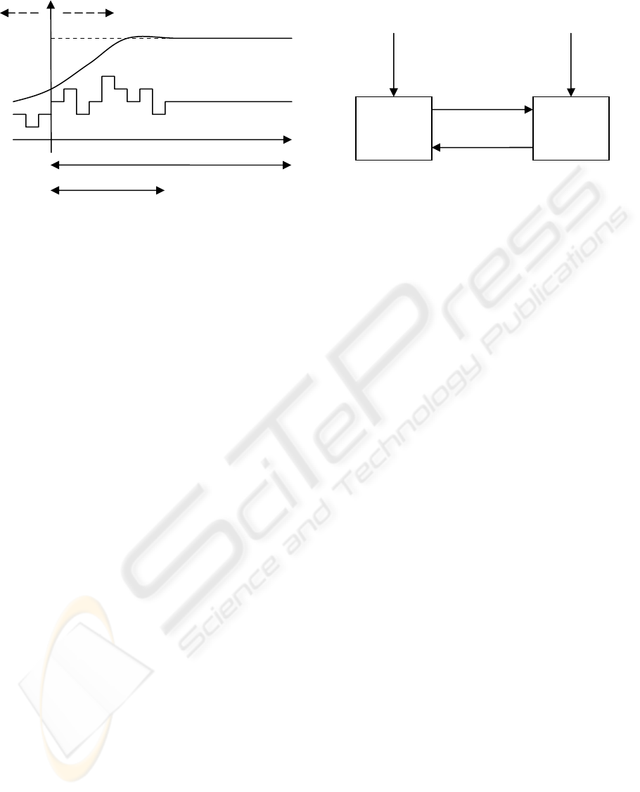
The algorithm consists of two main elements, an
optimization tool and a model of the system. The
optimizer contains a cost function with constraints
and receives a reference trajectory w(t) to which it
tries to lead the outputs as presented in Figure 1. The
actual forecasting in MPC is done with the model
which is used to predict future outputs ŷ(t) on the
basis of the previous inputs u
P
(t) and future inputs
u(t) the optimizer has solved as presented in Figure
1. These forecasts are then used to evaluate the
control and a next optimization on the horizon is
made. After all the control signals on the horizon are
evaluated, only the first control signal is used in the
process and the rest of the future control signals are
rejected. This is done because on the next optimizing
instant, the previous output from the process is
already known and therefore a new, more accurate
forecast can be made due to new information being
available. This is the key point in the receding
horizon technique as the prediction gets more
accurate on every step of the horizon but also is the
source of heavy computing in MPC. The receding
horizon technique also allows the algorithm to
handle long time delays. (Camacho and Bordons
2002)
2.1 Implementing the cost function
As presented in equation 1, the basic form of a MPC
cost function penalizes changes made in control
weighted with a certain parameter λ. This kind of
damping is not very suitable for controlling an
inventory or a supply chain due to the difficulty of
determining the parameter λ as it usually is either
the cost of change in inventory level or the cost of
change in ordering. On the other hand the parameter
λ cannot be disregarded as it results as minimum-
variance control which most definitely is not the
control desired. Another problem with the basic
form of MPC used in inventory control is the fact
that it penalizes the changes made in ordering and
not in inventory levels, which can cause unnecessary
variations in the inventory level as will be shown
later in this study.
In this study we present a more suitable way to form
the cost function used in a model predictive
controller. The problematic penalizing of changes in
the control is replaced with a similar way to the one
)
(
tw
)
(
ˆ
t
y
)
(
tu
In
pu
t H
o
riz
o
n
Pr
ed
i
c
ti
o
n H
o
riz
o
n
Pas
t
Future
Model
Optimization
)(tw
)(
ˆ
ty
)
(
tu
)(tu
P
Figure 1: The main idea and the implementation of MPC.
ICINCO 2004 - INTELLIGENT CONTROL SYSTEMS AND OPTIMIZATION
130

presented in, for example, (Lambert, 1987) and used,
for example, in (Koivisto et al., 1991). An inverted
discrete filter is implemented in the cost function so
that the resulting cost function can be written as
()
∑
=
−
⋅−=
2
1
2
1*
)(
ˆ
)()(
N
Ni
iyqPiyJ
(2)
, where y
*
(i) = Target output,
ŷ(i) = Predicted output
P(q
-1
) = Inverted discrete filter
P(q
The filter P(q
-1
) used can be written as
The filter P(q
()
-1
) = Inverted discrete filter
-1
) used can be written as
()
K
K
−−−
−−−
=
−−
−
21
2
2
1
1
1
1
1
pp
qpqp
qP
(3)
As can be seen, the number of tuneable parameters
can be reduced as the simplest form of the cost
function consists of only one tuneable parameter, p
1
which is used in the filter. Naturally the reduction of
tuneable parameters is a definite improvement it
self.
The dampening performed by the model reference
control is also an advantage concerning bullwhip
effect as over ordering has been found one of the
major causes of this problem. (Towill, 1996) When
the model reference control is applied to an
inventory level controller the most basic form of the
cost function results as
(
)
∑
=
−
⋅−=
2
1
2
1*
)(
ˆ
)()(
N
Ni
iIqPiIJ
(4)
, where I
*
(i) = Desired inventory level
Î(i) = Predicted inventory level
P(q
-1
) = Inverted discrete filter as in
equation (3)
3 SIMULATIONS
The simulations in this study were made using
MATLAB® and Simulink®. The goal in the
simulations was to show the advantages of a model
reference controller in inventory control compared
to a traditional model predictive controller. To
construct the simulators a set of universal supply
chain blocks was used. The main idea in these
blocks is the ability to construct any supply chain
desired without programming the whole chain from
scratch. The basic structure of a desired chain can be
implemented with basic drag and drop operations
and actual dynamics can be programmed afterwards.
The set of blocks consists of three different elements
which are inventory block, production block and a
so called dummy supplier block. These blocks are
the actual interface for programming each individual
element. With these blocks the whole supply chain
can be constructed and simulated with a high level
of visibility and clarity.
3.1 Simulator implementation tool
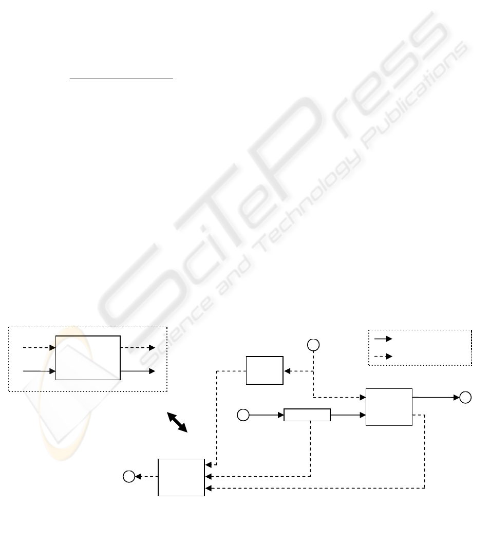
The main idea in the universal production block can
be seen in Figure 2. The submodules Stock, Control
and Demand forecast can all be implemented
Production
Inventory
Demand
Forecast
Control
Demand
Order
Inflow
Outflow
Material flow
Universal
production
block
Order Demand
Information flow
Inflow Outflow
Figure 2: Structure of the universal production block.
MODEL REFERENCE CONTROL IN INVENTORY AND SUPPLY CHAIN MANAGEMENT - The implementation of
a more suitable cost function
131

uniquely. For example the Inventory block can be
constructed to operate linearly in order to test more
theoretical control methods or it can even be
implemented as realistic as possible to study the
performance of a real world supply chain. The
inventory element represents an end product
inventory of a production plant. Also different
control and demand forecasting methods can be
tested and tuned via the Control and Demand
forecast elements in the block, respectively. The
universal production block has naturally a
submodule called Production which consists of
production dynamics in the simulated factory.
The universal inventory block is basically the
universal production block but without the
Production submodule. The universal inventory
block can be used as a traditional warehouse or as a
whole saler or even as a material inventory for a
production plant. As it consists of the same control
related elements as the universal production block, it
can have a control method and a inventory policy of
its own independently from the production plant.
The dummy supplier block is very different from the
rest of the set. It is used to solve the problem of long
supply chains. Usually one does not want to model
the whole supply chain as it can consist of tens of
companies. Most of the upstream companies are also
irrelevant in the simulations from the end products
point of view. Therefore it is necessary to replace
the companies in the upstream of the chain with a
dummy supplier block. This block takes the order
from its customer as an input and supplies this order
with certain alterations as an output. These
alterations can be anything from basic delay to
consideration of decay. Once again, this block can
be seen as an interface for the programmer who can
decide the actual operations within the block.
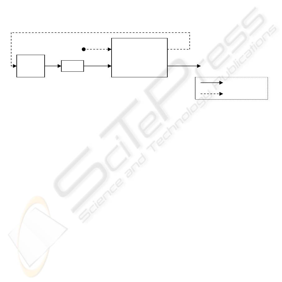
3.2 Inventory control simulations
To present the advantages in the model reference
control used in inventory control, a very simple
model was constructed using the universal block set
presented earlier. The structure of the simulator can
be seen in Figure 3. Both the universal production
block and the dummy supplier block are as
presented earlier. To keep the model as simple as
possible, all delays in the model are constant. Each
block in the model consists of a unit delay so that
total delay in the model is 3 units. Also no major
plant-model mismatch is involved in the controller
and no constraints are set. Both controllers also
receive identical accurate demand forecasts. With
this model we present two simulations with different
demand patterns.
Universal production
block
For the traditional model predictive controlled
inventory the following cost function was
implemented
(
) ()
∑
=
⎟
⎠
⎞
⎜
⎝
⎛
∆+−=
2
1
2
2
*
)()(
ˆ
)(
N
Ni
iOiIiIJ λδ
(5)
, where I
*
(i) = Desired inventory level
Î(i) = Predicted inventory level
∆O(i) = Change in order rate
δ, λ = Weight parameters
For model reference controlled inventory we used
the cost function presented in equation 4 with the
most basic form of the filter so that the only
parameter to tune is p
1
. As mentioned earlier, the
number of tunable parameters in model reference
control is reduced by one when compared to the
traditional model predictive control. This is obvious
when we look at the cost functions presented in this
Orde
r
Demand
OutflowInflow
Dummy
supplier
block
Delay
Material flow
Information flow
Figure 3: The structure of the simulator used in this study.
ICINCO 2004 - INTELLIGENT CONTROL SYSTEMS AND OPTIMIZATION
132

simulation, as the cost function used in model
reference controller has only one parameter p
1
instead of the two parameters, δ and λ included in
the model predictive controller.
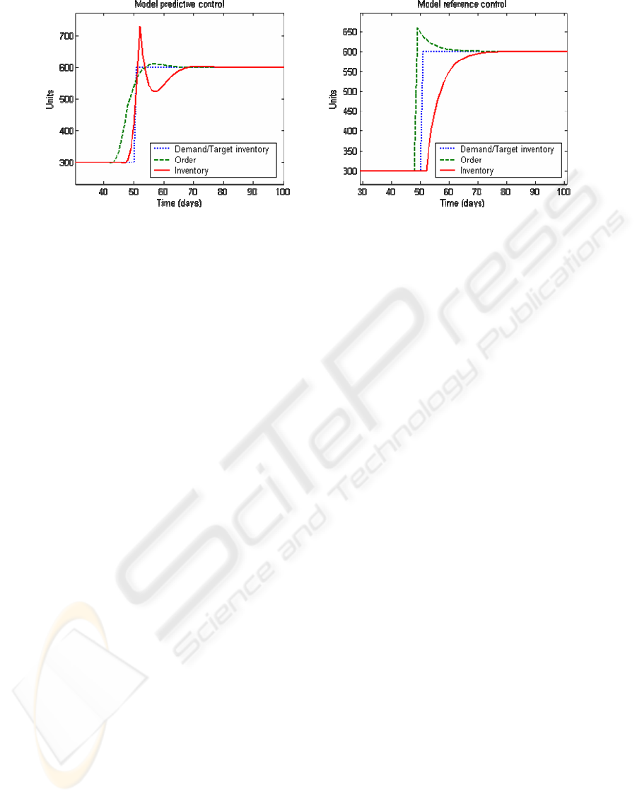
3.3 Step response simulations
The first simulation was a basic step response test
which demonstrated the difference between a model
refence controlled inventory and a traditional model
predictive controlled inventory. The step was
implemented in both demand and target inventory
levels at the same time to cause a major change in
the system. In other words, target inventory level
was set to follow the demand so that every day the
company had products in stock worth one day’s sale.
In this simulation the controller parameters were
chosen to be as follows: δ = 0.1, λ = 0.9 and p
1
=
0.8, with the control horizon of 10 days. The results
can be seen in Figure 4 where a step in demand has
occured at the moment of 50 days. As can be seen,
the response of the model reference controller is
much more smoother than the step response of a
traditional form of the model predictive controller.
This is due to the fact that the model reference
controller dampens directly the changes made in the
inventory level instead of dampening the changes
made in ordering. Model predictive controller is
forced to start ordering excessively in advance to the
step due to the limitations in changing the control
action. The more reasonably implemented model
reference controller orders exactly the amount
needed every instant. It becomes obvious that the
penalizing of control actions is not a suitable way to
control supply chain related tasks as it causes
additional variations in the system. Model reference
control is much more efficient in achieving what
was beeing pursued in this study – smooth control
method which is simple to tune and implement.
Figure 4: Step responses of an MPC-controlled inventory. In the left-hand figure the cost function is in the form
presented in equation 5, and in the right-hand figure the cost function is in the form presented in equation 4.
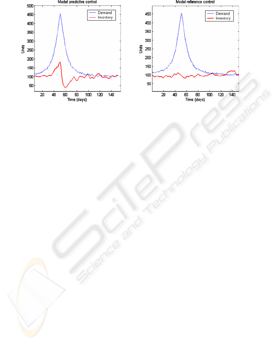
3.4 Simulations with a more realistic
demand pattern
A more practical simulation was also completed
with more realistic demand pattern and forecasting
error. The demand involved also noise which made
the control task even more realistic. The control
horizon was kept at 10 days in both controllers but
the parameters δ and λ needed to be retuned as the
parameters δ and λ used in the previous simulation
resulted as very poor responses. New parameters
were chosen as follows: δ = 0.3 and λ = 0.7. The
model reference controller did not need any retuning
as it survived both simulations very satisfyingly with
same parameter p
1
= 0.8. The target inventory level
was kept constant in the level of 100 units. This is
propably not the most cost efficient way of
managing an inventory but was used nevertheless to
keep the results easy to understand.
The demand curve and inventory response can be
seen in Figure 5. The demand curve is identical in
both pictures but as can be seen there were major
differences in inventory levels. Inventory levels in
the model predictive controlled case showed major
variations at the same time as demand rapidly
increased. No such variations were found in the
model reference case. Once again the penaling of
control actions forced the controller to order
excessive amounts in order to avoid stock-out.
MODEL REFERENCE CONTROL IN INVENTORY AND SUPPLY CHAIN MANAGEMENT - The implementation of
a more suitable cost function
133

4 CONCLUSIONS
In this study we presented a solution to the
problematic determining of the cost parameter
penalizing changes made in the control in model
predictive controller used in business related
systems. The model reference control was studied
and simulations performed to demonstrate the
abilities and advanteges of this control method. It
has been shown, that the model reference control
method is an effective way to control an inventory
and most of all that the method allows us to avoid
the problematic parameter λ in the equation 1. This
reduction of a very problematic parameter is most
definitely inevitable if any kind of practical solutions
are ever desired. Therefore all future research
concerning business related control should concider
this. It should also be kept in mind that any
reduction of tuneable parameters can be seen as an
advantage.
Also we showed in this study that the model
reference control is at least as applicable in
inventory control as model predictive control if not
even better. The simple, yet effective and smooth
response model reference control provides suits
perfectly to the unstable and variating environment
of business related systems. It can also be said that
the filter-like behaviour is desireable in order to
reduce the bullwhip behaviour, but further research
is needed on this field.
A new supply chain simulator interface was also
presented and used in the simulations of this study.
The set of universal supply chain blocks gives an
opportunity of testing and simulating the perforance
of different control methods or even different forms
of supply chains without reprogramming the basic
elements of inventory and production.
REFERENCES
Figure 5: The inventory responses of both controllers to a gaussian-shaped demand pattern.
Camacho, E. F. and Bordons, C., 2002, Model Predictive
Control.
Springer-Verlag London Limited
Hennet, J.-C., 2003. A bimodal scheme for multi-stage
production and inventory control. In Automatica, Vol
39, pp. 793-805.
Koivisto, H., Kimpimäki, P., Koivo, H., 1991. Neural
predictive control – a case study. In 1991 IEEE
International Symposium on Intelligent Control. IEEE
Press.
Lambert, E. P., 1987. Process Control Applications of
Long-Range Prediction. PhD Thesis, University of
Oxford. Trinity.
Maciejowski, J. M., 2002, Predictive Control with
Constraints. Pearson Education Limited
Rivera, D. E., Braun, M. W., Flores, M. E., Carlyle, W.
M., Kempf, K. G., 2003. A Model predictive control
framework for robust management of multi-product,
multi-echelon demand networks. In Annual Reviews in
Control, Vol. 27, pp. 229-245.
Towill, D. R., 1996. Industrial dynamics modeling of
supply chains. In International Journal of Physical
Distribution & Logistics Management, Vol. 26, No. 2,
pp.23-42.
Tzafestas, S., Kapsiotis, G., Kyriannakis, E., 1997. Model-
based predictive control for generalized production
problems. In Computers in Industry, Vol. 34, pp. 201-
210.
Ydstie, B. E., Grossmann, I. E., Perea-López, E., 2003, A
Model predictive control strategy for supply chain
optimization. In Computers and Chemical
Engineering, Vol 27, pp. 1202-1218.
ICINCO 2004 - INTELLIGENT CONTROL SYSTEMS AND OPTIMIZATION
134