
STABILIZING CONTROL FOR HIGHER ORDER SYSTEMS VIA
REDUCED ORDER MODEL- A PASSIVITY BASED APPROACH
B. Bandyopadhyay and Prashant Shingare
IIT Bombay
Mumbai, INDIA
H. K. Abhyankar
Vishwakarma Institute of Technology
University of Pune
Pune, INDIA
Keywords:
Odd and even polynomials, Lower order controller, System reduction, Passivity and Stability
Abstract:
In this paper a methodology for design of stabilizing control for high order system via reduced order model is
presented. In the first part a method is proposed for the reduction of original higher order passive system to
a lower order stable model, using this reduced order model, a strictly passive controller of order equal to that
of reduced order model is designed. It is shown that this lower order controller designed from reduced order
model when applied to original higher order system results in to close loop stability.
1 INTRODUCTION
The reduced model makes the synthesis and analysis
of controller simpler so the reduction of high order
systems to a reduced order system has been a topic of
interest of many researchers. However, the controller
designed from reduced order model do not guaran-
tee stability of resulting closed loop when it is ap-
plied to original higher order system. This problem of
guaranteed stabilization of original system has been
addressed by very few researchers such as (Bandy-
opadhyay et al, 1998), (Lamba and Rao, 1974), (Chi-
dambara and Schanker, 1974). In this paper a method-
ology for lower order controller design is proposed,
theory is developed to show that the lower order sta-
bilizing passive controller designed for the reduced
model by proposed method stabilizes original passive
system.
The rest of the paper is organized as follows: Sec-
tion 2 reviews theory of passivity and passivity based
control. In Section 3 the conditions are derived under
which the given lower order controllers are strictly-
passive. In Section 4 new methods for passive system
reduction preserving stability is presented with two
numerical examples. In Section 5, new methodology
for low-order controller design is described and based
on this methodology a numerical example of low or-
der controller design for higher order system is illus-
trated followed by conclusion.
2 THEORY OF PASSIVITY
In this section we will review the theory of passiv-
ity (Guillemin, 1957)-(Yengst, 1964),(Braess, 2003),
(Van Der Schaft, 1999), (Lozano-leal and Joshi,
1988), (Wen, 1988), (Lozano-leal and Joshi, 1990)
and (Tao and Ioannou, 1990). For a given transfer
function it is possible to synthesize the network using
the passive circuit components only if the given trans-
fer function satisfy certain conditions. These condi-
tions are known as the realizability conditions for the
given transfer function. Any transfer function is real-
izable iff
• Numerator and denominator polynomials are Hur-
witz.
• The given transfer function is positive real.
2.1 Positive real function
In this sub-section we will state various definitions,
theorem and corollary related to the positive real func-
tion (Lozano-leal and Joshi, 1990; Tao and Ioannou,
1990).
Definition 1 : Let H(s) be a rational function
1. If H(s) is positive real, then it has no poles and
zeros in C
+
2. Any pole and zero on the imaginary axis is simple
and have positive real residue.
122
Bandyopadhyay B., Shingare P. and Abhyankar H. (2004).
STABILIZING CONTROL FOR HIGHER ORDER SYSTEMS VIA REDUCED ORDER MODEL - A PASSIVITY BASED APPROACH.
In Proceedings of the First International Conference on Informatics in Control, Automation and Robotics, pages 122-129
DOI: 10.5220/0001141201220129
Copyright
c
SciTePress
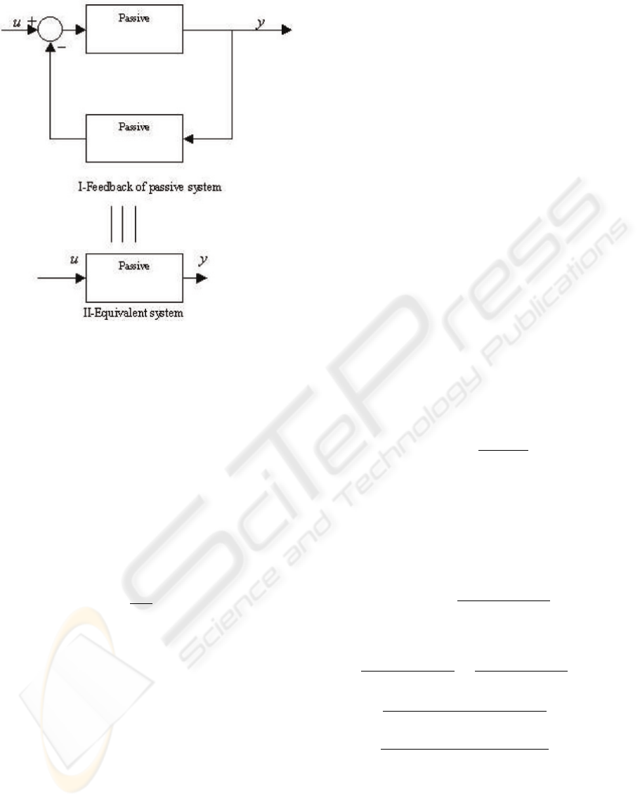
Figure 1: Feedback interconnection of passive systems and
their Equivalence
3. The function H(s) is positive real iff it has no poles
in C
+
and Re(H(jω)) ≥ 0 for all ω ∈ R .
Definition 2 : A rational transfer function H(s)
is strictly positive real function iff
1. All elements of H(s) are analytic in Re(H(jω))
2. H(jω)+H
∗
(jω) 0 for all ω ∈ R .
3. Strong definition imposes condition as
lim
ω→∞
ω
2
(H(jω)+H
∗
(jω)) 0
Theorem 1 : A positive real function Z(s)
cannot have any poles or zeros in the r. h. s. plane. j
axis poles of Z(s) and
1
Z(s)
must be simple with real
positive residues.
Theorem 2 : If Z(s) is prf, the degree of the
numerator cannot differ from that of the denominator
by more than unity.
2.2 Passivity based stabilizing
control
Any system H(s) satisfying Definition 1 or Defini-
tion 2 is passive system. Passivity based control is
a methodology which consist in controlling a system
with the aim at making the closed loop system, pas-
sive(M. Vidyasagar, 1983).
Theorem 3 : Consider two passive systems
interconnected as shown in Figure 1. If one of the
system is strictly passive and another strong strictly
passive then the resulting close loop system will
always be stable.
This theorem allows a passivity based stability
analysis(M. Vidyasagar, 1983). Alternatively it can
be stated that a negative feedback loop consisting of
two passive systems is passive(Sepulchre et al, 1997).
3 LOWER ORDER PASSIVE
CONTROLLERS
In this section we will derive the conditions under
which the lower order controller is strictly passive.
We will restrict this discussion to third order con-
troller. These conditions are extremely important in
the design of lower order controller using the pro-
posed method of controller synthesis. For the deriva-
tion of these condition we are referring the spr condi-
tion given in definition 2.
3.1 First order system
Conditions under which a first order system is spr are
simple as it has only three parameters. Let the system
be of the form
C
1
(s)=
x
0
y
0
+ y
1
s
(1)
for this system to be spr the necessary and sufficient
condition are met by x
0
,y
0
and y
1
being greater than
zero.
3.2 Second order system
Let the second order strictly proper system be
C
2
(s)=
x
0
+ x
1
s
y
0
+ y
1
s + y
2
s
2
(2)
The C
2
(s) will be spr if (C
2
(jω)C
∗
2
(jω)) > 0 for all
ω ∈ R i. e
x
0
+ x
1
s
y
0
+ y
1
s + y
2
s
2
+
x
0
− x
1
s
y
0
− y
1
s + y
2
s
2
> 0
2x
0
y
0
+2(x
0
y
2
− x
1
y
1
)s
2
y
2
0
+2y
2
y
0
s
2
+ y
2
2
s
4
− y
2
1
s
2
> 0
2x
0
y
0
+2(x
1
y
1
− x
0
y
2
)ω
2
y
2
0
+(y
2
1
− 2y
2
y
0
)ω
2
+ y
2
2
ω
4
> 0
This condition will be true when both the numerator
and denominator are of the same sign. We are restrict-
ing ourselves to the case when all the coefficients of
the controller are greater than zero. Thus, conditions
satisfying above inequality are x
0
,x
1
,y
o
,y
1
and y
2
be
positive with
x
1
y
1
≥ x
0
y
2
and y
2
1
≥ 2y
2
y
0
(3)
STABILIZING CONTROL FOR HIGHER ORDER SYSTEMS VIA REDUCED ORDER MODEL - A PASSIVITY
BASED APPROACH
123

3.3 Third order controller
Let the system be of the form
C
3
(s)=
x
0
+ x
1
s + x
2
s
2
y
0
+ y
1
s + y
2
s
2
+ y
3
s
3
(4)
Now again by spr definition, the conditions under
which the C
3
(s) is spr are
0 <y
0
,y
1,
y
2
,y
3
,x
0,
x
1
and x
2
(5)
x
1
y
1
>y
0
x
2
+ y
2
x
0
,
x
2
y
2
>x
1
y
3
y
2
1
≥ 2y
2
y
0
y
2
2
≥ 2y
1
y
3
4 A NEW MODEL ORDER
REDUCTION TECHNIQUE
An approximation that is frequently used is the Pade
technique. The approximated model by Pade tech-
nique matches first 2r time moments with the original
higher order system, where r is the order of the re-
duced model. However, the Pade approximation does
not guarantee the stability of the reduced model. This
problem is addressed in (Shamash, 1975) and over-
come by Routh-Pade approximation technique. In
this method reduced model matches only initial r time
moments with the original system thus compromising
with the accuracy of the fit. In (Lepschy and Viaro,
1982) an improvement to this method is suggested to
improve the accuracy of the fit, but method is cumber-
some and in few cases it’s possible to perfectly match
only one additional time moment and approximately
matching another. In this section a new method is pro-
posed to reduce the order of a linear time invariant
higher order stable system, using the Hermite-Biehler
stability theorem and Pade approximation. The pro-
posed method not only tackle the problem of the guar-
anteed stability but it can match additional time mo-
ments over the conventional Routh-Pade method.
4.1 The order reduction problem
Let the transfer function of a higher order linear time
invariant stable system is given by
G(s)=
a
0
+ a
1
s + a
2
s
2
+ ···+ a
n−1
s
n−1
b
0
+ b
1
s + b
2
s
2
+ ···+ b
n
s
n
(6)
The order of the original higher order system is n. We
want a reduced order model of order r. Thus, the prob-
lem is to find the approximated reduced order model
of order r such that it matches two additional time mo-
ments while preserving the stability.
4.2 Matching additional time
moments
Let G(s) be the transfer function of a higher order
linear time invariant stable system. Let D(s) be the
denominator polynomial of order n and N(s) is the
numerator polynomial of order (n − 1). Then denom-
inator and numerator of equation 6 can be expressed
as
N(s)=a
0
+ a
1
s + a
2
s
2
+ ···+ a
n−1
s
n−1
D(s)=b
0
+ b
1
s + b
2
s
2
+ ···+ b
n
s
n
These polynomials can be separated into even and odd
parts as follows (Bhattacharya et al, 1995), For n odd
D
even
(s)=b
0
+ b
2
s
2
+ b
4
s
4
+ ···+ b
n−1
s
n−1
D
odd
(s)/s = b
1
+ b
3
s
2
+ b
5
s
4
+ ···+ b
n
s
n−1
For n even
D
even
(s)=b
0
+ b
2
s
2
+ b
4
s
4
+ ···+ b
n
s
n
D
odd
(s)/s = b
1
+ b
3
s
2
+ b
5
s
4
+ ···+ b
n−1
s
n−2
Let (0 ± ω
d
e,i
) and (0 ± ω
d
o,i
) denotes the roots of
the D
even
(s) and D
odd
(s)/s respectively. Then for
the stable plant, by interlacing property, the following
condition must be satisfied(Bhattacharya et al, 1995),
0 <ω
d
e,1
<ω
d
o,1
<ω
d
e,2
<ω
d
o,2
<ω
d
e,3
··· (7)
This concept of interlacing of roots of even and odd
polynomials is used to construct a reduced degree sta-
ble denominator polynomial as follows:
Write D
even
(s) and D
odd
(s) in term of their roots
ω
d
e,1
,ω
d
e,2
··· and ω
d
o,1
,ω
d
o,2
, ···For n even
D
even
n
(s)=
n/2
i=1
(s
2
+ ω
2
de,i
)
D
odd
n
(s)/s =
n/2−1
i=1
(s
2
+ ω
2
de,i
)
Now if we want to obtain a reduced r
th
order model,
then the even and odd polynomials for the reduced
order denominator polynomial can be written as, for
r even
D
even
r
(s)=
r/2
i=1
(s
2
+ ω
2
de,i
) (8)
D
odd
r
(s)/s =
r/2−1
i=1
(s
2
+ ω
2
de,i
)
Using (8) a modified reduced denominator can be
constructed as
D
rm
(s)=K
1
D
even
r
(s)+K
2
D
odd
r
(s) (9)
ICINCO 2004 - SIGNAL PROCESSING, SYSTEMS MODELING AND CONTROL
124

Where K
1
and K
2
are real numbers and should have
same sign so that the denominator polynomial is inter-
lacing and hence stable. Then the higher order system
given by equation (6) can be approximated by r
th
or-
der system as
G
hb
(s)=
x
0
+ x
1
s + x
2
s
2
+ ···+ x
r−1
s
r−1
y
0
+ y
1
s + y
2
s
2
+ ···+ y
r
s
r
(10)
Now, we know that
D
rm
(s)=K
1
r/2
i=1
(s
2
+ ω
2
de,i
)
+K
2
s
r/2−1
i=1
(s
2
+ ω
2
de,i
)
= y
0
+ y
1
s + y
2
s
2
+ ···+ y
r
s
r
Now, the problem becomes finding (r +2)unknown
coefficients of reduced model given in (10), this prob-
lem is addressed here with the help of Pade approx-
imation. Let the original higher order system, given
by equation (6), be represented as
G(s)=c
0
+ c
1
s + ···+ c
r
s
r
+ c
r+1
s
r+1
+ ··· (11)
Now, taking the power series expansion of the re-
duced model given by equation (10), around s =0
and equating equal powers of s we get
x
0
= y
0
c
0
(12)
x
1
= y
0
c
1
+ y
1
c
0
x
2
= y
0
c
2
+ y
1
c
1
+ y
2
c
0
x
r−1
= y
0
c
r−1
+ y
1
c
r−2
+ ···+ y
r−1
c
0
0=y
0
c
r
+ y
1
c
r−1
+ y
2
c
r−2
+ ···+ y
r
c
0
:
:
0=y
0
c
r+2
+ y
1
c
r+1
+ ···+ y
r−1
c
r−1
Where, C
i
s are the coefficient of the equation (11)
above. The above set of equations can be written in
matrix form as
c
r
c
r−1
.. c
1
c
r+1
c
r
.. c
2
c
r+2
c
r+1
.. c
r−1
⎡
⎢
⎣
y
0
y
1
:
y
r−1
⎤
⎥
⎦
=
⎡
⎢
⎣
−c
0
−c
1
:
−c
r−1
⎤
⎥
⎦
(13)
And
c
0
0 .. 0
c
1
c
0
.. 0
c
r−1
c
r−2
.. c
0
⎡
⎢
⎣
y
0
y
1
:
y
r−1
⎤
⎥
⎦
=
⎡
⎢
⎣
−x
0
−x
1
:
−x
r−1
⎤
⎥
⎦
(14)
It must be noted that in the above transformation of
equation (12) to (14) that y
r
=1. The solutions to
the equations (13) and (14) gives the coefficients of
the reduced r
th
order model for the given n
th
order
system.
Now, suppose that given higher order system is to
be reduced to a 3
rd
order system. Then even and odd
parts of denominator can be written as
D
even
r
(s)=(s
2
+ ω
2
de,1
)
D
odd
r
(s)/s =(s
2
+ ω
2
do,1
)
Hence, from equation (9)
D
rm
(s)=K
1
(s
2
+ ω
2
de,1
)+K
2
s(s
2
+ ω
2
do,1
)
D
rm
(s)=K
1
ω
2
de,1
+ K
2
ω
2
do,1
s + K
1
s
2
+ K
2
s
3
This gives guaranteed stability for any value of K
1
and K
2
such that ratio K
1
/K
2
is positive. Then
this parameterized equation can be used to match two
additional time moments exactly and approximately
match the third.
D
rm
(s)=b
0
+ b
1
s + b
2
s
2
+ b
3
s
3
So we have, b
0
= K
1
ω
2
de,1
,b
1
= K
2
ω
2
do,1
,b
2
= K
1
and b
3
= K
2
. Observe that b
0
and b
2
are linear com-
bination of K
1
, where as b
1
and b
3
are linear combi-
nation of K
2
. Lets assume ω
2
de,1
to be unknown. Then
using constraint optimization equations (13) and (14)
can be solved for K
1
,K
2
and ω
2
de,1
such that
F = −b
0
c
5
+ b
1
c
4
+ b
2
c
3
− b
3
c
2
is minimum and the solution set satisfy the constraints
for stability, that is, K
1
and K
2
have same sign and
0 <ω
d
e,1
<ω
d
o,1
, which ensure the Hermite-Beihler
stability of denominator polynomial as interlacing is
preserved. Then (r+2) moments of the approximated
system will exactly match with the original higher or-
der system while (r +3)
rd
will match approximately.
Under this condition the reduced third order model
will exactly match initial five time moments where as
matching 6
th
time moment will be matched approxi-
mately . The reduced 3
rd
order model is given by
G
3
hbr
(s)=
x
0
+ x
1
s + x
2
s
2
y
0
+ y
1
s + y
2
s
2
+ y
3
s
3
4.3 Numerical Examples
In this section we will consider two most critical ex-
amples taken in from literature.
4.3.1 Numerical Example 1
Let us consider an example where ordinary Pade ap-
proximation technique results in to an unstable model,
while the method described gives directly a stable re-
duced model. The original fourth order system is
given by
G(s)=
100 + 395s + 527s
2
+ 267s
3
1+4s +6s
2
+4s
3
+ s
4
(15)
STABILIZING CONTROL FOR HIGHER ORDER SYSTEMS VIA REDUCED ORDER MODEL - A PASSIVITY
BASED APPROACH
125
we will reduce this system to third order model. Now
G(s) can be expressed as
H(s) = 100 − 5s − 53s
2
+ 109s
3
− 198s
4
+ ···
The denominator of the original higher order system
is
D(s)=1+4s +6s
2
+4s
3
+ s
4
We can write the polynomial in to even and odd parts
as following
D(s)=(1+6s
2
+ s
4
)+(4s +4s
3
)
=(s
2
+5.828)(s
2
+0.1715) + 4s(s
2
+1)
separating this in to even and odd parts
D
even
(s)=(s
2
+5.828)(s
2
+0.1715)
D
rodd
(s)/s =(s
2
+1)
It can be easily observed that the system is stable
as even and odd roots of this polynomial interlace ie
0 < (0.4141 = ω
de,1
) < (1 = ω
do,1
) < (2.4141 =
ω
de,2
). Now the stable denominator of the reduced or-
der approximation can be obtained by using equation
(9) as,
D
rm
(s)=K
1
(s
2
+ ω
2
de,1
)+K
2
s(s
2
+ ω
2
do,1
)
D
rm
(s)=K
1
ω
2
de,1
+ K
2
ω
2
do,1
s + K
1
s
2
+ K
2
s
3
Putting ω
2
de,1
=0.1715 and solving equations (13)
and (14) under the required stability constraints on we
get K
1
=3.418,K
2
=1and ω
2
do,1
=2.7686. We
have 3rd order reduced model as
G
PR
(s)=
58.53 + 273.93s + 298.037s
2
0.5853 + 2.7686s +3.429s
2
+ s
3
(16)
This model matches initial 5-time moments exactly
where as 6
th
time moment is matched approximately
with the original system. Where as, the approximated
model by Routh-Pade method for the same system is
obtained and is given by
G
RP R
(s)=
100 + 176.25s +62.937s
2
1+1.8125s +1.25s
2
+0.3125s
3
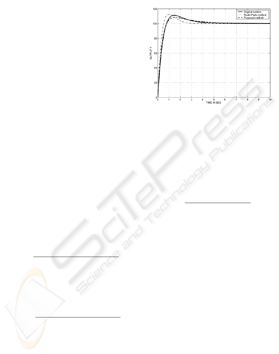
The step responses of original higher order system,
approximated model by proposed method, approxi-
mated model by Routh-Pade method are plotted in
Figure 2. From the response it is clear that proposed
method performs good than the conventional Routh-
Pade method and it matches 2 more time moments
exactly and one approximately over the Routh-Pade
method, which matches only initial 3 time moments
with the original system.
Figure 2: Step responses of original and approximated sys-
tems
4.3.2 Numerical Example 2
Now, Consider one more critical example suggested
by A. Lipschy and U. Viaro(Lepschy and Viaro,
1982), where classical Pade approximation results
into an unstable model and proposed method in to
more appropriate reduced stable model. The original
higher order system is given by
G(s)=
2+8s +8s
2
+12s
3
1+2s +12
2
+4s
3
+2s
4
Where
H(s) = 100 − 5s − 53s
2
+ 109s
3
− 198s
4
+ ···
The denominator of the original higher order system
is
D(s)=1+2s +12s
2
+4s
3
+2s
4
We can write the polynomial in to even and odd parts
as following
D(s)=(1+12s
2
+2s
4
)+(2s +4s
3
)
=(s
2
+5.915)(s
2
+0.085) + 2s(2s
2
+1)
splitting this in to even and odd parts
D
even
(s)=(s
2
+5.915)(s
2
+0.085)
D
rodd
(s)/s =(2s
2
+1)
It can be easily observed that the system is stable as
even and odd roots of this polynomial interlace i.e.
0 < (0.085 = ω
2
de,1
) < (0.5=ω
2
do,1
) < (5.915 =
2
ω
de,2
). Now the stable denominator of the reduced or-
der approximation can be obtained by using equation
(9) as
D
rm
(s)=K
1
(s
2
+ ω
2
de,1
)+K
2
s(s
2
+ ω
2
do,1
)
D
rm
(s)=K
1
ω
2
de,1
+ K
2
ω
2
do,1
s + K
1
s
2
+ K
2
s
3
ICINCO 2004 - SIGNAL PROCESSING, SYSTEMS MODELING AND CONTROL
126
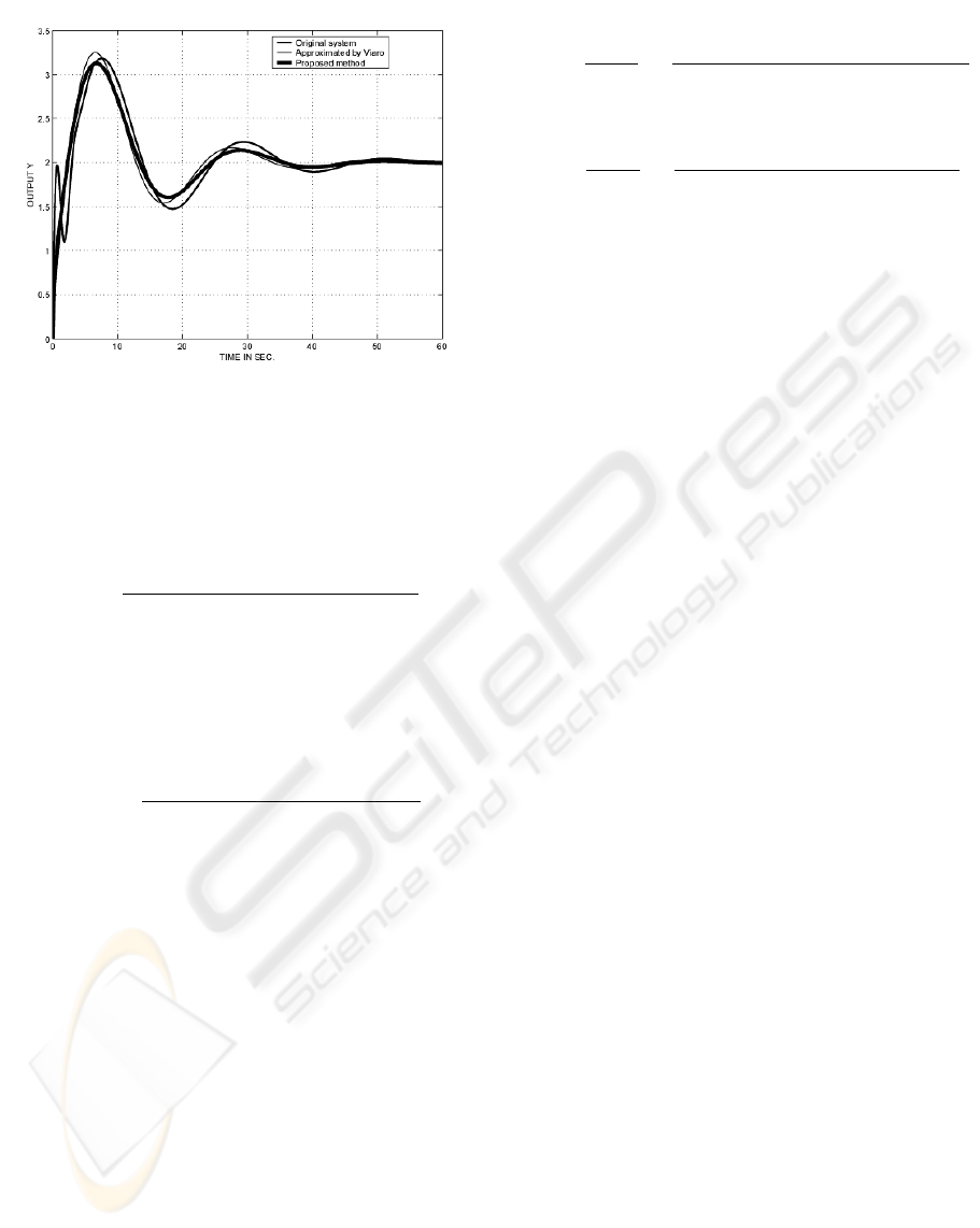
Figure 3: Step responses of original and approximated sys-
tems
Putting the values of K
2
=1,ω
2
de,1
=0.085, us-
ing Pade equations(14) and (13)We have 3rd order re-
duced model as
G
hb
(s)=
0.626 + 2.7504s +2.8502s
2
0.313 + 0.7492s +3.6872s
2
+ s
3
This model matches initial 5-time moments exactly
where as 6
th
time moment is matched approximately
with the original system. The approximated model by
improved Routh-Pade method for the same system is
obtained(Lepschy and Viaro, 1982), given by
G
RP R
(s)=
2+8.7309s +7.4618s
2
1+2.3654s +11s
2
+4.3853s
3
The step responses original higher order system, ap-
proximated model by proposed method, approxi-
mated model by Routh-Pade method are plotted in
Figure 3. From these plots it is clear that proposed
method performs good even than the improved Routh-
Pade method proposed by U. Viaro, it matches 1 more
time moment exactly and another time moment ap-
proximately, over the improved Routh-Pade method,
which matches only initial 4 time moments with the
original system.
5 DESIGN OF LOW ORDER
CONTROLLER
In this section an approach to design low order con-
troller from reduced order model of the original plant
is described. This method gives r
th
order controller
for n
th
order plant, that is, the order of the controller
is equal to the reduced order of the plant.
Let the controller be of the form
C
r
(s)=
N
c
(s)
D
c
(s)
=
x
0
+ x
1
s + x
2
s
2
+ .. + x
r−1
s
r−1
y
0
+ y
1
s + y
2
s
2
+ .. + y
r
s
r
(17)
and let the reduced order model be
G
r
(s)=
N
r
(s)
D
r
(s)
=
c
0
+ c
1
s + c
2
s
2
+ .. + c
r−1
s
r−1
d
0
+ d
1
s + d
2
s
2
+ .. + d
r
s
r
(18)
Then, the characteristics equation of the closed loop
is as
Q(s)=N
c
(s)N
r
(s)+D
c
(s)D
r
(s) (19)
let it be in the following form
(s
2
+ λ
1
s + λ
2
)(s
r
+ α
1
s
r−1
+ α
2
s
r−2
+ ···+ α
r
)
(20)
where λ
1
and λ
2
are free variables greater than zero
while α
1
,α
2
....α
r
can be fixed. Equating the coeffi-
cients of s we obtain the coefficients of C
r
(s) in terms
of λ
1
and λ
2
as
[A][B]=[C]
1
λ
1
λ
2
(21)
where A is (2
r+1
)×(2
r+1
) non singular matrix whose
inverse exist, B is (2
r+1
)×1 matrix and C is (2
r+1
)×
3 matrix and are given by
A =
⎡
⎢
⎢
⎢
⎢
⎢
⎢
⎣
d
r
000. 0
d
r−1
d
r
00. 0
d
r−2
d
r−1
c
r−1
0 . 0
......
......
000.c
0
c
1
000. 0 c0
⎤
⎥
⎥
⎥
⎥
⎥
⎥
⎦
B =
⎡
⎢
⎢
⎢
⎢
⎢
⎢
⎣
y
r
y
r−1
y
r−2
.
.
x
1
x
0
⎤
⎥
⎥
⎥
⎥
⎥
⎥
⎦
and
C =
⎡
⎢
⎢
⎢
⎢
⎢
⎢
⎣
100
α
1
10
α
2
α
1
1
...
...
0 α
r
α
r−1
00α
r
⎤
⎥
⎥
⎥
⎥
⎥
⎥
⎦
In this way the coefficients of controller are obtained
in terms of λ
1
and λ
2
,the free variables. Now we can
choose these two parameters in such a way that the
resulting controller is spr system. Thus, when it is
applied to the original higher order passive system it
will stabilize it.
STABILIZING CONTROL FOR HIGHER ORDER SYSTEMS VIA REDUCED ORDER MODEL - A PASSIVITY
BASED APPROACH
127

5.1 Numerical example
Here will consider a numerical example for the design
of lower order controller using the proposed method,
where a higher order system is reduced using the pro-
posed methods. We will use proposed method of or-
der reduction. Design a third order controller for a PR
system given by
G(s)=
100 + 395s + 527s
2
+ 267s
3
1+4s +6s
2
+4s
3
+ s
4
Here we have to design a third order controller. The
order of controller designed by proposed method is
equal to the order of the model, so we will reduce the
given system to third order model. Using this model
a third order spr controller can be designed.
In previous section, we have reduced this system
given by equation (15) to a third order model given
by equation (16), the reduced model is
G
r
(s)=
58.53 + 273.93s + 298.03s
2
0.5883 + 2.7686s +3.429s
2
+ s
3
Here, the reduced model is stable. Now, we will de-
sign a stabilizing strictly passive controller for this
model. Let the controller be of the form
C
3
(s)=
N
c
(s)
D
c
(s)
=
x
0
+ x
1
s + x
2
s
2
y
0
+ y
1
s + y
2
s
2
+ y
3
s
3
Then the characteristics equation of the closed loop
becomes
Q(s)=N
c
(s)N
r
(s)+D
c
(s)D
r
(s)
Let it be equal to
(s
2
+ λ
1
s + λ
2
)(s
4
++α
1
s
3
+ α
2
s
2
+ α
3
s + α
4
)
lets assume that the four fixed closed loop poles to
be at -1, -2, -3, -4. This gives α
1
=10,α
2
=35,
α
3
=50,α
4
=24. Thus from equation(21) we have
A =[
A
1
A
2
]
A
1
=
⎡
⎢
⎢
⎢
⎢
⎢
⎢
⎣
1000
3.429 1 0 0
2.769 3.429 1 298
0.585 2.769 3.429 1
00.588 2.769 3.429
000.588 2.769
0000.588
⎤
⎥
⎥
⎥
⎥
⎥
⎥
⎦
A
2
=
⎡
⎢
⎢
⎢
⎢
⎢
⎢
⎣
000
000
000
58.53 298 0
58.53 273.9 298
058.03 273.9
0058.03
⎤
⎥
⎥
⎥
⎥
⎥
⎥
⎦
and
C =
⎡
⎢
⎢
⎢
⎢
⎢
⎢
⎣
100
10 1 0
35 10 1
50 35 10
24 50 35
02450
0024
⎤
⎥
⎥
⎥
⎥
⎥
⎥
⎦
we get
y
3
=1
y
2
=6.5710 + λ
1
y
1
=26.77 − 65.75λ
1
+ 301.66λ
2
y
0
= −0.05 + 0.24λ
1
− 1
x
2
=0.3375 − 1.05λ
1
+3.48λ
2
x
1
= −0.2691 + 1.07λ
1
− 4.11λ
2
x
0
=0.0006 − 0.0025λ
1
+0.4238λ
2
Here free parameters λ
1
and λ
2
can be chosen such
that the resulting controller is passive. Thus by re-
ferring the passivity condition for third order system
given by equation(5) and choosing these two free vari-
ables λ
1
and λ
2
(both positive) to be λ
1
=0.4 and
λ
2
=0.03 we get
y
3
=1,y
2
=6.97,y
1
=9.519,y
0
=0.0095
x
2
=0.018,x
1
=0.6359,x
0
=0.0123
Thus the third order spr controller obtained is
C
3
(s)=
N
c
(s)
D
c
(s)
=
0.0123 + 0.6359s +0.018s
2
0.009 + 9.519s +6.97s
2
+ s
3
(22)
This low order strictly passive controller designed
from the reduced order model will stabilize the model
and the original higher order passive system.
6 CONCLUSION
Most modern robust controller design methods nor-
mally result in a complex controller. The controller
so designed generally has an order atleast equal to
that of the original system. Thus, the reduction of
high order system to a lower order model is neces-
sary. However, the reduced order model must cap-
ture the essential properties of the original higher or-
der system. In control system design stability of the
system is most important where as least possible er-
ror estimate is preferred. Here in this paper, this is-
sues is addressed by developing an improved method
for system reduction. From the illustrated examples
it is observed that reduced model by this method not
only preserve the stability but also has same dynamic
response.
If a controller is designed from the reduced model,
it does not guarantee the close loop stability when it
ICINCO 2004 - SIGNAL PROCESSING, SYSTEMS MODELING AND CONTROL
128

is applied to the original system. In this the higher
order system is reduced to a lower order model. A
stabilizing passive low order controller for the sta-
ble reduced order model is designed, which when ap-
plied to original higher order passive system results
in a stable closed loop. Though, the proposed method
is applied for the order reduction in this paper, any
stability-preserving system reduction method can be
applied for this purpose.
REFERENCES
R. Sepulchre, M. Jankovic, and P. V. Kokotovic, (1997).
Constructive nonlinear control, communication and
control engineering. Springer-Verlag London.
E. A. Guillemin, (1957). Synthesis of passive networks New
York, NY: Jhon Willey and Sons Inc.
D. Hazony, (1963).Elements of network synthesis.Reinhold
Publishing Corporation, Newyork.
B. Peikari, (1974). Fundamentals of network analysis and
synthesis. Prentice Hall, Englewood Cliffs, New Jer-
sey.
W. C. Yengst, (1964). Procedures of modern network syn-
thesis.Collier-Macmillan Limited, London.
G. Obinata and B. D. O. Anderson, (2001). Model reduc-
tion for control system designSpringer-Verlag London
Limited.
S. P. Bhattacharya, H. Chapellat and L. H. Keel,(1995).Ro-
bust control: the parametric approach. Upper Saddle
River,Prentice-Hall PTR.
B. Bandyopadhyay, Unbehauen and B. M. Patre, (1998).
A new algorithm for compensator design for higher
order system via reduced model. Automatica Vol. 34,
No. 7.
G. Schmitt-Braess, (2003). Feedback of passive sys-
tems:synthesis and analysis of linear robust control
systems. IEE Proc.-Control Theory Apply., Vol. 150,
No. 1.
S. S. Lamba and S. V Rao, (1974). On suboptimal control
via the simplified model of the Davison. IEEE Trans.
Automat. Control,AC-9, pp 448-450.
M. R. Chidambara and R. B. Sancher, (1974). Low order
Generalized Aggrigated Model and Suboptimal Con-
trol.IEEE Trans. on Automat. Control., April 1975, pp
175-180.
A. J. van der schaft, (1999),
2
-Gain and passivity tech-
niques in nonlinear control, communication and con-
trol engineering. Springer-Verlag, Heidelberg, 2nd
edition.
R. Lozano-leal and S. M. Joshi, (1988), On the design
of dissipative LQG-type controllers, Proceedings of
the 27th conference on decision and control, Austin,
Texas.
B. Bandyopadhyay and H. Unbehauen, (1999), Interval sys-
tem reduction using kharitnov polynomials. In Euro-
pean control conference, Karlsruhe, Germany.
Y. Shamash, (1974). Stable reduced order model using pade
type approximation. In IEEE Trans. Automatic Con-
trol, AC-19, pp. 615-616.
Y. Shamash, (1975). Model Reduction using the Routh Sta-
bility Criterion and the Pade Approximation Tech-
nique.In Int. J. Control, Vol. 21, No. 3,475-484.
M. F. Hutton and B. Friedland, (1975). Routh approxima-
tion for reducing order of linear time invariant sys-
tem.In IEEE Trans. on Automatic Control, AC-20, pp.
329-337.
John T. Wen, (1988). Time domain and frequency domain
conditions for strict positive realness. In IEEE Trans.
on Automatic control, Vol. 33, No. 10.
R. Lozano-Leal and S. M. Joshi, (1990). Strictly positive
real transfer functions revisited.In IEEE Trans. on Au-
tomatic control, Vol. 35, No. 11.
G. Tao and P. A. Ioannou, (1990). Necessary and sufficient
conditions for strictly positive real matrices. In IEE
Proc. on Control Theory and Apply., Vol. 137, Oct.
1990, pft G. No 5, pp 360-366.
N. K. Sinha and W. Pille, (1971).A new method for reduc-
tion of dynamic systems. In Int. J. of Control, Vol. 14,
No. 1,111-118.
N. K. Sinha and Kuszta, (1983). Modelling and Identifi-
cation of Dynamic Systems. New York Van Nostrand
Reinhold, Ch. 8 pp 133-164.
A. Lepschy and U. Viaro, (1982). An improvement in the
Routh-pade approximation technique. In Int. J. Con-
trol, Vol. 36, No. 4,643-661.
M. Vidyasagar, (1983). Nonlinear systems. Prentice Hall,
Engle Wood Cliffs, New Jersey.
P. Shingare, B. Bandyopadhyay and H. K. Abhyankar,
(2003), Model order reduction technique based on in-
terlacing property and pade approximation. In Pro-
ceedings of 27th National Systems Conference, IIT
Kharagpur, India, pp 50-54.
P. Shingare and H. K. Abhyankar, (2003). Hermite-
Biehler Method for System Reduction Preserving Sta-
bility. In Proceedings of International Conference on
CAD/CAM, Robotics and Autonomous Factories, IIT
Delhi, India.
STABILIZING CONTROL FOR HIGHER ORDER SYSTEMS VIA REDUCED ORDER MODEL - A PASSIVITY
BASED APPROACH
129
