MATLAB MODELS OF ACMS IN CONTROL SYSTEMS

Fei Hao, Fei Xia, E. Graeme Chester, Alex Yakovlev, Ian G. Clark

School of Electronic, Electrical and Comuter Engineering, University of Newcastle upon Tyne

Keywords: ACM, MATLAB, Stateflow, Distributed Control

Abstract: Asynchronous communication mechanisms (ACMs) are poten

tially useful in systems with heterogeneous

timing as data connectors between processes belonging to different timing domains. In distributed,

concurrent and embedded digital systems, there is often a desire to have some temporal decoupling between

different parts of a system. ACMs provide a means with which concurrent processes can communicate with

one another and yet still avoid synchronization. This paper describes efforts to implement MATLAB-based

models of existing ACM algorithms. These techniques will facilitate the inclusion of ACMs in such

application fields as distributed control and signal processing systems.

1 INTRODUCTION

Inter-process asynchrony is inevitable for

computation networks in the future, firstly because

different and diverse functional elements, especially

those connecting to analogue domains, tend to have

different timing requirements (Kelly et al 2003,

Simpson 2003), and secondly because concurrent

and distributed system implementations lead to

greater asynchrony between components as

semiconductor technology advances and the degree

of integration increases (ITRS 2003 “Design”

document emphasizes multiple clock domains and

source-synchronous signalling and predicts networks

of self-timed blocks). The size of computation

networks is becoming larger, and the traffic between

the processing elements is increasing. Handling the

data communications which make up the traffic,

therefore, may determine much of the performance

and characteristics of such systems.

In truly distributed system

s such as sensor

networks (Kelly et al 2003, Min et al 2001)[1, 4],

there is often a desire to have temporal decoupling

of various kinds between digital processes. For

instance, parts of a distributed control system may

consist of control laws mapped onto hardware

embedded into parts of the plant environment, whilst

the higher hierarchies of the system may be

implemented with software running in general

purpose processors which are shared multitasking

units. It can be very important to have temporal

decoupling between these two parts of the control

algorithm at the hardware level because of such

reasons as avoiding deadlock propagation through

the system, the desire to have low power

characteristics in remote and battery powered units,

the physical impossibility of keeping everything

synchronized in distributed systems, different parts

of a system requiring radically different processing

speeds, etc.

Asynchronous communication mechanisms

(AC

Ms) have been investigated since the 1980s and

have by now developed into a coherent field

including classification, specification, and

techniques for implementation, analysis and

verification (Simpson 2003, Xia et al 2002). ACMs

are potentially useful in systems with heterogeneous

timing as data connectors between processes

belonging to different timing domains, which may

exist either out of necessity or desirability. They can

also be useful as digital mimics for various types of

data connections in analogue systems, with different

types of ACMs suiting different data requirements.

ACM classification was successfully expanded to

include types providing more qualitative asynchrony

and richer data properties than the traditional FIFO

buffer. This made it clear that these applications can

be envisaged. The successful work in synthesis and

verification of implementations made them practical

(Simpson 2003, Xia et al 2002).

An ACM, as defined here, is a connector

etween two asynchronous processes, a writer and a

reader, through which a sequence of data items can

be passed (Simpson 2003, Xia et al 2002) [2, 5]. The

general scheme of these kinds of data

communication mechanisms is shown in Figure 1.

Most ACM implementations tend to include shared

memory, accessible to both writer and reader, for the

Hao F., Xia F., Chester G., Yakovlev A. and Clark I. (2004).

MATLAB MODELS OF ACMS IN CONTROL SYSTEMS.

In Proceedings of the First International Conference on Informatics in Control, Automation and Robotics, pages 54-61

DOI: 10.5220/0001141700540061

 SciTePress

data being transferred, and control variables, each of

which is usually set by one side and read by the

other.

ACMs emphasize the asynchrony between the

reader and writer processes during data transfer, and

are therefore especially suitable for systems of the

future where multiple time domains not fully

synchronized with one another predominate. ACMs

can be classified into four types according to the

qualitative properties of the inter-process

asynchrony during data transfer as shown in Table 1.

When discussing ACMs, we assume that the data

being transferred consists of a stream of items of the

same type, and the writer and reader processes are

single-thread loops, during each cycle of which a

single item of data is transferred to or from the

ACM.

Table 1: ACM classification

NRR RR

NOW BB RR-BB

OW OW-BB OW-RR-BB

In Table 1, which follows the tradition of 2x2

matrix classification schemes found in (Simpson

2003, Xia et al 2002), NRR and RR stand for non-

rereading and rereading, while NOW and OW mean

non-overwriting and overwriting. Whether rereading

is permitted determines if the reader may be held up

waiting for new data to appear in the ACM. Whether

overwriting is permitted determines if the writer may

be held up waiting for previous data in the ACM to

be accessed by the reader. Therefore, a BB or

bounded buffer without overwriting and rereading

provisions, which includes most traditional inter-

process data buffering schemes, may require either

process to wait under certain circumstances. An RR-

BB may require the writer to wait when previous

data items have not been read. An OW-BB may

require the reader to wait when no newer data has

been made available by the writer after the previous

read. An OW-RR-BB, however, does not require

either side to wait under any circumstances.

The study of ACMs so far, though extensive, has

not extended to their direct modelling in application-

level tools. Previous proposals for modelling ACMs

at a higher level, treating them as components in

larger systems, have employed Petri nets (Xia 2000).

This was suitable for the case where systems

containing ACMs can be regarded and analysed as

general discrete event digital systems. However, in

order to study the effect of including ACMs in such

engineering application systems as control systems,

especially when analogue parts are present, ACM

models need to be integrated into popular

application-level tools such as MATLAB.

2 STATEFLOW MODELS OF

ACMS

MATLAB is a widely used modelling, simulation

and analysis tool for engineering application systems

in such fields as control, signal processing, large

scale hybrid systems with analogue and discrete

parts, etc. It also includes a Stateflow facility with

which discrete state-transition subsystems such as

ACMs can be modelled. In order to broaden the

application space of ACMs, we have developed a

method to model and simulate ACMs using

MATLAB, based on Stateflow. The two examples in

this section illustrate the method with RR-BB

algorithms.

2.1 Represent Handshake in the

Stateflow Model

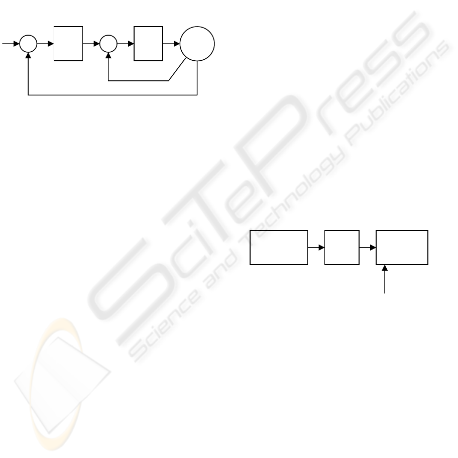
The progress of ACM algorithms can be controlled

by the writer and reader processes via request-

acknowledgement handshakes. A four phase

handshake protocol follows this order: sending a

request, waiting for the acknowledgement sent from

the other side, releasing (resetting) the request, and

resetting the acknowledgement from the other side.

This can be modelled in Stateflow as shown in

Figure 2. One handshake cycle is represented in the

following way: a request is generated in the state

entry actions (the “En” statements), which are

executed when entering the state; the state itself

represents waiting for the acknowledgement in the

transition conditions (the conditions in the square

brackets, in the case of Figure 2, ACK becoming 1),

which lead to the exit from the state (end of waiting)

and executions of the transitions; on exiting a state,

the requests are released (in the “Ex” statements);

and then the acknowledgements can be reset.

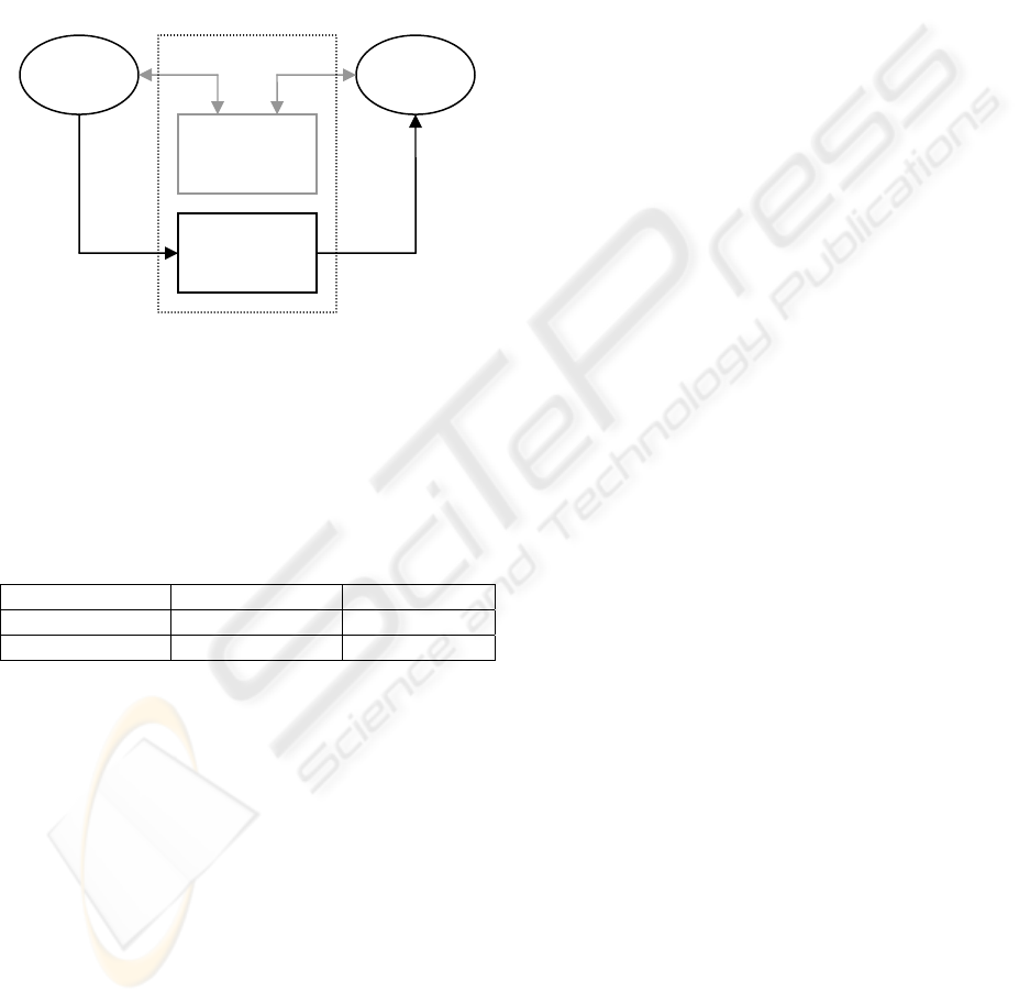
Reade

Write

Shared

memory

Control

variables

ACM

data data

Figure 1: ACM with shared memory and possibly

control variables

MATLAB MODELS OF ACMS IN CONTROL SYSTEMS

We built the Stateflow models of ACMs. based

on this representation of the handshake protocol.

2.2 Global View of RR-BB ACM

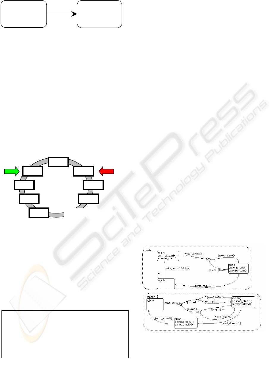
A Bounded Buffer (BB) ACM can be implemented

with a ring structure formed by identical memory

cells (see Figure 4). One cell stores one data item at

a time. The cells can be added or removed to change

the size of the buffer. The two arrows in the figure

indicate the reader pointer and the writer pointer.

Each pointer points to the cell which is being

accessed by its corresponding process. After the

completion of a data access, the reader and writer

pointers are moved forward according to the specific

algorithm.

If the writer cycle is much longer than that of the

reader, its pointer may point to the cell immediately

ahead of the reader pointer. In this case the buffer is

empty, i.e. all the data items in the buffer have

already been read by the reader. Conversely, if the

writer cycle is much shorter than the reader cycle, its

pointer will likely point to the cell just behind the

reader pointer. The buffer is full in this case and

none of the data items in the buffer have been read

by the reader.

Rereading, if permitted, only occurs when the

buffer is empty with a new read request arriving.

Overwriting, if permitted, only happens when the

buffer is full with a new write request coming.

En:req2=1;

Ex:req2=0;

En:req1=1;

Ex:req1=0;

[ACK1==1]

The RR-BB ACM allows rereading but not

overwriting. A multi-cell RR-BB algorithm is

described in Figure 3.

Figure 3: Handshake protocol in Stateflow

Here n is the number of free cells which are not

occupied by the pointers w and r. Therefore for this

algorithm, n+2 is the total number of the memory

cells in the ring.

The algorithm can be implemented based on the

handshake protocol. For instance, each cycle of the

writer part of the algorithm can be connected to the

external writer process through a handshake during

each cycle of operation (i.e. request from writer

process to start wr, acknowledged by the writer part

of the algorithm at the end of w0). This also applies

to the reader side. The relationships between

statements rd and wr and the cell memory can also

be modelled as such handshakes. Both the writer and

reader algorithm cycles have wait states from which

they emerge only when the condition is correct

(external request arrives and additionally in the

writer’s case, r becoming different from w).

Cell

Cell Cell

Cell

Cell Cell

Cell

…

Cell

Figure 5 shows the Stateflow model for the

algorithm in Figure 3. In the writer, the wr statement

is matched to the writing state because it handshakes

with the shared memory. The w0 statement, which

updates w, is mapped to the transition action after

the writing state. After updating w, the write cycle is

completed and the done state handshakes with the

environment. The ww statement is merged into the

idle state, which represents waiting for the next

cycle request from the external writer, because it is

also conditional waiting. The two wait conditions

are “AND-ed” to produce the equivalent result.

Figure 4: Ring organization of ACM buffer

In the reader, what r0 does is modelled in the

transition actions before the reading state. The rd

statement is mapped to the reading state because of

the handshake. A done state follows reading to

acknowledge to the environment the completion of

var w: 0..n+1; r: 0..n+1; initialized sensibly (e.g.

r=w-1) and initialize data in the cells.

Writer Reader

wr:write cell w; r0:if (r+1 mod n+1)≠w

w0:w:=(w+1 mod n+1); then r:=(r+1 mod n+1);

ww:wait until r≠w; rd: read cell r;

Figure 5: Stateflow Model for Algorithm in Figure 2

Figure 2: n+2 Cells RR-BB ACM algorithm

ICINCO 2004 - SIGNAL PROCESSING, SYSTEMS MODELING AND CONTROL

the read cycle. An idle state is added at the end to

wait for the next request.

The initial state in the writer part is w_idle. The

writer will not become active until the write request

(the request signal from the external writer wishing

to start a write data access – statement wr) comes

and w is not the same as r. When the writer becomes

active, a write_start signal is sent to the cells, in

order to write the new data item to the corresponding

cell. When the writer receives a write_done signal

from the buffer, indicating the completion of wr, it

will change w to point to the next cell. Because of

the ring configuration, the writer needs to check if

the current cell is the one with the highest index. If it

is, w will be set to 0, which is the cell with the

lowest index. Otherwise, the value w will simply be

incremented. After that, a write_ack is sent back to

the environment. Then the writer will wait for the

resetting of the write_req signal before going back to

the w_idle state.

The reader is similar to the writer. The initial state

is r_idle. When a read request comes from the

environment, the reader will check if the next cell is

occupied by the writer or not. The same r+1 mod n+1

exercise is carried out to determine the index of the

next cell (either r+1 or 0). If the next cell is occupied

by the writer, the reader pointer will remain at the

current cell (for rereading). If not, the reader pointer

will be moved forward according to the r+1 mod n+1

rule. Then the reader sends a read_start signal to the

buffer in order to read the data item in the

corresponding cell. On completion of reading, the

reader will receive a read_done signal from the cells. A

read_ack is sent to the environment, and then the active

state moves to the r_idle state waiting for the next

read_req signal.

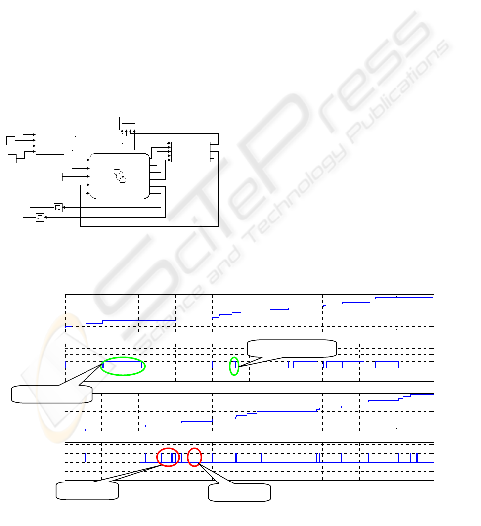
This Stateflow model can be plugged into the

Simulink environment. This is shown in Figure 7.

The test environment generates write requests, read

requests and the input data items. The data path is

made of memory slots (one slot per cell) to which the

data items are written in and from which the data items

are read out.

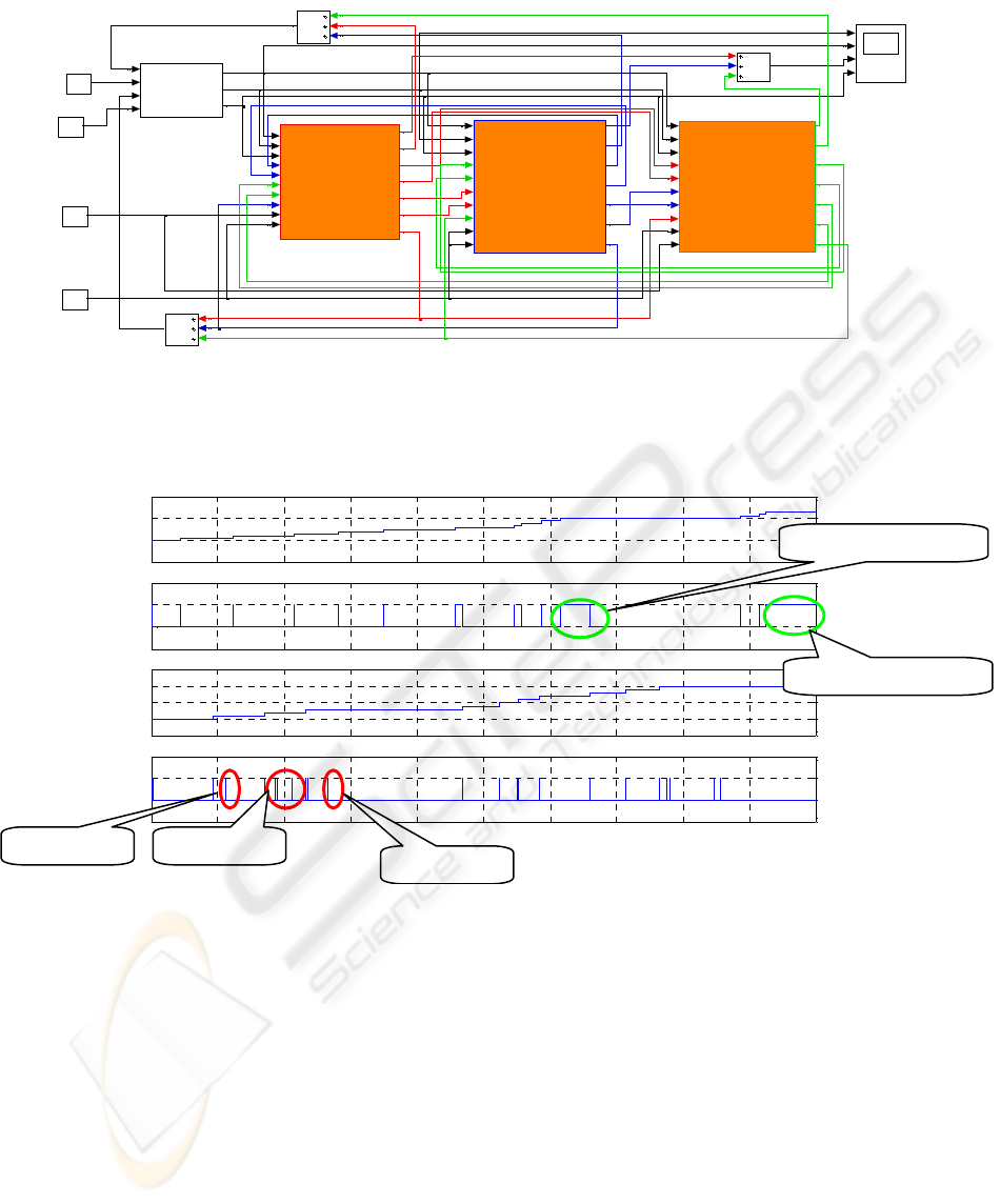
This ACM was simulated in this environment, with

resulting waveforms shown in Figure 6. Rereading

occurred when read requests came without new data

items available, as in the case after the data items 4 and

5 were read (encircled in the diagram). In this

simulation, n was set to 1, i.e. the total number of cells

was 3. Therefore, the writer waited if two consecutive

data items have not been read, as in the case after items

3 and 8 were written (encircled in the diagram).

Wac k

W_M u

Rac k

R_Mu

Wr eq

Dat a

Rre q

Test Environment

Sco pe

Number

Memory1

Memory

Dat ai n

Write_start

Read_start

Dat aO ut

Write_done

Read_done

Data Path

writ e_req

read_req

writ e_done

read_done

write_start

read_start

writ e_ack

read_ack

Control Ci r cuit

-C-

Constant1

-C-

Constant

Output Data

Write request

Input data

Read request

The algorithm in Figure 3, though neat and easily

understandable, is not suitable for hardware

implementation. In particular, the integer control

variables w and r will need many protections in order

to be considered atomic. The global view nature of the

indexing also means that the actual setting and reading

Figure 6: The Model in Figure 5 with Test Environment

0 5 10 15 20 25 30 35 40 45 50

Input data

0 5 10 15 20 25 30 35 40 45

-1

Writ e request

0 5 10 15 20 25 30 35 40 45 50

Output Data

5 10 15 20 25 30 35 40 45

-1

Read request

Wait after Item 8

Wait after Item 3

Time

RR Item 4

RR Item 5

Figure 7: Simulation Waveforms for Figure 6

MATLAB MODELS OF ACMS IN CONTROL SYSTEMS

of these variables will include multiplexing and de-

multiplexing on a scale depending on the number n.

The fork and join operations needed mean that an

implementation of n+3 cells, for instance, cannot be

easily built upon one of n+2 cells.

2.3 Modular Design Model

The cellular structure of this kind of buffered ACMs

suggests that it may be possible to construct a

standard individual cell, complete with its own local

control variables, then use n of these for an n-cell

solution. This modular design approach is much

better suited for hardware implementations.

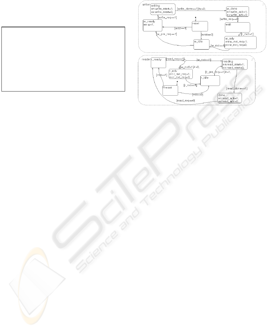
A localized algorithm for a single cell is

described in Figure 9.

The action “advancing to next cell” causes the

end of execution of the current cell’s writer/reader

algorithm and the beginning of the next cell’s one

from wr/r0. The reader algorithm loops at the same

cell until the condition wnext=0 is met. The writer

will wait at a cell until the condition rnext=0 is met.

Note that the writer algorithm sets both w and wnext

and reads rnext, and the reader algorithm sets both r

and rnext and reads wnext.

Because of the existence of the action “advance

to next”, one more handshake is in the writer/reader

in addition to the two mentioned in the previous

algorithm. After the writer/reader has advanced to

the next cell, the current one enters an idle state, and

it cannot respond to external requests until the

current w/r is set again (the process completing a

cycle of the ring). This needs to be dealt with using

an additional state in the model.

Figure 8 shows the Stateflow model of the

algorithm in Figure 9. In the writer part, the wr and

w0 statements were represented in Stateflow in the

same way as in Figure 3. After the w_done state, a

wait state is used to represent the ww statement,

instead of being merged into the following state. The

reasons of doing that are: 1) releasing the write

request is the only condition of finishing a write

cycle; 2) the only prerequisite of advance is r in the

next cell having been reset. These two conditions

cannot be combined together. The next statement wa

was mapped to the w_adv state. w_idle and w_ready

represented the two different states mentioned

before.

var w: 0..1; r: 0..1; initialized sensibly (one cell

has w=1 and one has r=1, all others being 0) and

initialize data in the cells.

Writer Reader

wr: write; r0: if wnext=0 then

w0: w:=0; wnext:=1; begin r:=0; rnext:=1;

ww: wait until

rnext=0;

advance to next end

wa: advance to next; rd: read;

Figure 9: Modular Design RR-BB ACM Algorithm

Figure 8: Stateflow model of the algorithm in Figure 9

The reader part consists of the three handshake

states, the idle and the ready state.

The model worked as follows: when the write

pointer points to the current cell (and with current

w=1) and a write request comes, the writer writes the

input data item into the memory of the cell. After

that, w is reset to 0 and wnext set to 1. At this point,

the write cycle is finished, a write acknowledgement

is sent back to the environment. However, the writer

pointer will not move to the next cell until rnext

becomes 0.

When a read request comes, the reader firstly

checks if the next cell is occupied by the writer or

not (if wnext is 1 or not). If it is not, it moves the

pointer to the next cell and does the reading.

ICINCO 2004 - SIGNAL PROCESSING, SYSTEMS MODELING AND CONTROL

Wack

W_ Mu

Rack

R_Mu

Wreq

Dat a

Rreq

Test Environment

Scope

write_req

Dat ain

read_req

w_nxt

r_nxt

w_pre_req

r_pre_req

nxt_rd_ack

wrst

rrst

Dat aOut

write_ack

w_nxt_req

r_nxt_req

read_ack

RR BB Single2

write_req

Dat ain

read_req

w_nxt

r_nxt

w_pre_req

r_pre_req

nxt_rd_ack

wrst

rrst

Dat aOut

write_ack

w_nxt_req

r_nxt_req

read_ack

RR BB Single1

write_req

Dat ain

read_req

w_nxt

r_nxt

w_pre_req

r_pre_req

nxt_rd_ack

wrst

rrst

Dat aOut

write_ack

w_nxt_req

r_nxt_req

read_ack

otherwise, it stays the current cell and rereads its data

item.

The ready states in the Stateflow are used to

initialise the position of the pointers. If the pointer

moves to the current cell, the system is in the ready

state, otherwise, it is in the idle state.

Consider the control flow from w_ready state to

w_done state in the writer: After releasing the

acknowledgement, the writer does not send the advance

request until r_nxt = 0 (next cell is no longer accessed

by the reader). When the writer receives the w-setting

acknowledgement from the next cell, it releases the

request, moves to the idle state, and waits for the

advance request from the previous cell.

When a read request comes to the current cell, the

reader sends an advance request to the next cell if it is

no longer accessed by the writer (w_nxt is not 1), and

goes to the idle state when r in the next cell is set. At

the same time, the next cell moves the active state from

idle to reading. After finishing reading, the reader

sends an acknowledgement and goes back to the ready

state.

The Simulink model showing connections between

cells is in Figure 10. Figure 11 shows the simulation

results for the model in Figure 10. Rereading occurred

after data items 1, 2, 3 were read, and writer waiting

happened after data items 9, 12 were written. These

correspond with the properties specified for the RR-BB

ACM.

RR BB Single

Constant3

Constant2

-C-

Constant1

-C-

Constant

Figure 10: Modular 3 Cell RR-BB ACM Simulink model

0 5 10 15 20 25 30 35 40 45 50

-10

0 5 10 15 20 25 30 35 40 45 50

-1

0 5 10 15 20 25 30 35 40 45 50

-5

0 5 10 15 20 25 30 35 40 45 50

-1

Time

Input Data

Write Reqs

Output Data

Read Reqs

Wait after Item 9

Wait after Item 12

RR Item 1 RR Item 2

RR Item 3

Figure 11: Simulation of the RR-BB ACM model in Figure 10

MATLAB MODELS OF ACMS IN CONTROL SYSTEMS

3 A MOTOR CONTROL SYSTEM

WITH ACM

Here we use an example application system case

study to demonstrate the usefulness of these kinds of

ACM models.

Figure 12 shows the basic structure of a

distributed motor control system found in (Kappos et

al 1990). The vC and iC blocks are the velocity and

current/torque controllers, both integrated into the

same ASIC in (Kappos et al 1990). The velocity and

current control laws are implemented digitally.

Because of the different speed requirements (the

inner loop requiring considerably faster control

actions than the outer one), the digital parts of the

ASIC controller were implemented in a dual-speed

fashion. The link between vC and iC is in effect

implemented as an analogue connection, with the

digital output from vC first converted into analogue

then re-sampled to provide the input for iC.

This kind of temporal decoupling is essential in

these kinds of distributed systems. In motor control

systems especially, if the inner and outer loops are

not temporally decoupled, potential digital hazards

such as deadlocks can propagate through from one

loop to another. The function of the inner control

loop is normally safety-critical, because even

temporary failure there could have catastrophic

effects such as causing the power electronic

elements or fuses to fail. If such a motor is used in a

safety-critical application (for instance in an

aeroplane fuel pump), such failures which cannot be

recovered on-line must always be avoided. As a

result, the capability of the inner loop to continue

functioning even when the outer loop has stopped

working is of vital importance. This means that even

though both vC and iC may be integrated into the

same piece of silicon, they must in reality be

temporally independent of each other.

Because of the difference in speed requirements

for the vC and iC parts, assuming the same

technology is being used to implement them in

hardware, the part of the hardware where vC is

implemented could have large amounts of excess

computational capacity. This makes it attractive to

attempt to make use of this capacity for other tasks,

i.e. to effectively implement the vC part as one of

the threads in a multi-tasking processing element.

This makes it possible for its progress to be affected

by other factors outside the immediate control

system boundary. Well-implemented operating

systems such as real-time kernels may take care of

the safety-critical implications of such complications

by ensuring that critical threads do not wait for

information from other threads.

At the basic hardware level of the data

connection between the iC and vC parts of an

embedded hard-wired controller chip, this kind of

non-blocking communication can be implemented

by using an analogue link. However, this implies an

analogue/digital hybrid chip.

- -

M iC vC

With ACMs, the same kind of temporal

decoupling can be realized without resorting to

inserting an analogue wire between two digital

devices. The OW-RR-BB type ACMs, especially,

mimics this function of an analogue wire perfectly.

When an OW-RR-BB is “full”, the writer overwrites

one of the items in it instead of waiting for a space

to appear, and when it is “empty” the reader rereads

the item it read during the previous cycle instead of

waiting for a new item to appear. This is

functionally the same as connecting the writer with

the reader through a D/A and A/D converter pair,

assuming perfect level-matching in the converters.

Figure 12 Schematic of dual-loop motor control system

We have implemented a Stateflow OW-RR-BB

ACM model using the techniques outlined in the

previous section. It was then inserted into a

MATLAB model of the system in Figure 12.

Figure 13 shows the way in which an OW-RR-

BB ACM was used to connect the fast and slow

controllers in the motor control system. The iC part

of the control law has a sampling frequency of 30

kHz and the vC part of the control law has a

sampling frequency of 1 kHz. Our simulations with

a single-cell OW-RR-BB ACM show that the reader

part of the ACM reads each data item approximately

30 times, as expected, and overwriting rarely

occurred. Some artificial perturbations were put into

the frequencies of the clock signals going into both

the vC and iC parts as a form of noise.

iC – fast ACM

i feedback

vC – slow

Figure 13: ACM connecting fast and slow circuits

The simulation results were compared with

results from simulating an entirely analogue version

of the same system. There were no detectable

differences from the output waveforms of both θ and

i. This is expected because an OW-RR-BB ACM is

ICINCO 2004 - SIGNAL PROCESSING, SYSTEMS MODELING AND CONTROL

the digital emulation of direct analogue connection,

if the latency/delay associated with the buffering can

be neglected. It behaves the same as a D/A →

perfect analogue connection with delay → A/D

combination in this case. Because of the vastly faster

inner loop the latency caused by the buffering

associated with the single cell in the ACM is

unimportant.

4 SUMMARY AND FUTURE

WORK

We have developed a series of techniques with

which MATLAB/Simulink models can be

implemented for ACM algorithms. Initial simulation

results show that these models perform as expected,

i.e. the same as predicted theoretically from the

algorithms.

An initial case study successfully demonstrated

that these kinds of ACM models can be plugged into

MATLAB models of control systems for the purpose

of simulation.

MATLAB direct to hardware fast prototyping

tools are becoming available (Xilinx), potentially

making it possible to save the step of implementing

DSP hardware through the traditional VLSI process.

Future developments in this direction could

potentially lead to the direct hardware

implementation of application systems containing

ACMs designed and verified in MATLAB. This

provides another motivation for this kind of work.

Future work includes the further development of

MATLAB/Simulink models for non-ACM

components which would highlight the effect of the

various degrees of temporal decoupling ACMs bring

to systems.

ACKNOWLEDGEMENT

This work is part of the Coherent project

(

http://async.org.uk/coherent) at the Newcastle

University supported by the EPSRC grant

(GR/R32666). The authors benefited from extensive

discussions with H. Simpson and E. Campbell and

wish to express our gratitude.

REFERENCES

Kelly, C. IV, V. Ekanayake, and R. Manohar, 2003.

SNAP: a sensor-network asynchronous processor.

Proc. ASYNC 2003, IEEE Computer Press.

Simpson, H., 2003. Protocols for Process Interaction. IEE

Proceedings on Computers and Digital Techniques,

2003, 150, (3), pp 157-182.

ITRS 2003.

http://public.itrs.net/files/2003itrs/home2003.htm.

Min, R. et al., 2001. Low-power wireless sensor networks.

Proc. VLSI Design 2001, January 3-7, 2001,

Bangalore, India.

Xia, F., A.V. Yakovlev, I.G. Clark, and D. Shang, 2002.

Data Communication in Systems with Heterogeneous

Timing,

IEEE Micro, 22, (6), pp. 58-69.

Xia, F., 2000. Supporting the MASCOT method with Petri

net techniques for real-time systems development.

PhD Thesis, London University.

Kappos, E., D.J. Kinniment, P.P. Acarnley, A.G. Jack,

1990. Design of an integrated circuit controller for

brushless DC drives. Proc. Fourth International

Conference on Power Electtronics and Variable-Speed

Drives, pp.336-341, London, UK, July 1990.

Xilinx System Generator for DSP,

http://www.xilinx.com/xlnx/xil_prodcat_product.jsp?ti

tle=system_generator

MATLAB MODELS OF ACMS IN CONTROL SYSTEMS