DEAD RECKONING FOR MOBILE ROBOTS USING TWO

OPTICAL MICE

Andrea Bonarini

Matteo Matteucci

Marcello Restelli

Department of Electronics and Information – Politecnico di Milano

Piazza Leonardo da Vinci, I-20133, Milan

Keywords:

Optical sensors, dead redoking, cinematic independent odometry, . . .

Abstract:

In this paper, we present a dead reckoning procedure to support reliable odometry on mobile robot. It is

based on a pair of optical mice rigidly connected to the robot body. The main advantages are that: 1) the

measurement given by the mice is not subject to slipping, since they are independent from the traction wheels,

nor to crawling, since they measure displacements in any direction, 2) this localization system is independent

from the kinematics of the robot, 3) it is a low-cost solution. We present the mathematical model of the sensor,

its implementation, and some empirical evaluations.

1 INTRODUCTION

Since the very beginning of mobile robotics, dead

reckoning was used to estimate the robot pose, i.e.,

its position and its orientation with respect to a global

reference system placed in the environment. Dead

reckoning is a navigation method based on measure-

ments of distance traveled from a known point used

to incrementally update the robot pose. This leads to

a relative positioning method, which is simple, cheap

and easy to accomplish in real-time. The main disad-

vantage of dead reckoning is its unbounded accumu-

lation of errors.

The majority of the mobile robots use dead reckon-

ing based on odometry in order to perform their navi-

gation tasks (alone or combined with other absolute

localization systems (Borenstein and Feng, 1996)).

Typically, odometry relies on measures of the space

covered by the wheels gathered by encoders which

can be placed directly on the wheels or on the engine-

axis, and then combined in order to compute robot

movement along the x and y-axes and its change of

orientation. It is well-known that odometry is subject

to:

• systematic errors, caused by factors such as

unequal wheel-diameters, imprecisely measured

wheel diameters and wheel distance, or an impre-

cisely measured tread (Borenstein and Feng, 1996);

• non-systematic errors, caused by irregularities of

the ﬂoor, bumps, cracks or by wheel-slippage.

In this paper, we present a new dead reckoning

method which is very robust towards non-systematic

errors, since the odometric sensors are not coupled

with the driving wheels. It is based on the mea-

sures taken by two optical mice ﬁxed on the bottom

of the robot. We need to estimate three parameteres

(∆x, ∆y, ∆θ), so we cannot use a single mouse, since

it gives only two independent measures. By using two

mice we have four measures, even if, since the mice

have a ﬁxed position, only three of these are indepen-

dent and the fourth can be computed from them. We

have chosen to use optical mice, instead of classical

ones, since they can be used without being in contact

with the ﬂoor, thus avoiding the problems of keeping

the mouse always pressed on the ground, the prob-

lems due to friction and those related to dust deposited

in the mechanisms of the mouse.

In the following section, we will present the moti-

vations for using this method for dead reckoning. In

Section 3, we show the geometrical derivation that al-

lows to compute the robot movement on the basis of

the readings of the mice. Section 4 describes the main

characteristics of the mice and how they affect the ac-

curacy and the applicability of the system. In Sec-

tion 5, we report the data related to some experiments

in order to show the effectiveness of our approach. Fi-

nally, we discuss related works in Section 6 and draw

conclusions in Section 7.

Bonarini A., Matteucci M. and Restelli M. (2004).

DEAD RECKONING FOR MOBILE ROBOTS USING TWO OPTICAL MICE.

In Proceedings of the First International Conference on Informatics in Control, Automation and Robotics, pages 87-94

DOI: 10.5220/0001143000870094

 SciTePress

2 MOTIVATIONS

The classical dead reckoning methods, which use

the data measured by encoders on the wheels or on

the engine-axis, suffer from two main non-systematic

problems: slipping, which occurs when the encoders

measure a movement which is larger than the actually

performed one (e.g., when the wheels lose the grip

with the ground), and crawling, which is related to a

robot movement that is not measured by the encoders

(e.g., when the robot is pushed by an external force,

and the encoders cannot measure the displacement).

Our dead reckoning method, based on mice read-

ings, does not suffer from slipping problems, since

the sensors are not bound to any driving wheel. Also

the crawling problems are solved, since the mice go

on reading even when the robot movement is due to a

push, and not to the engines. The only problem that

this method can have is related to missed readings due

to a ﬂoor with a bad surface or when the distance be-

tween the mouse and the ground becomes too large

(see Section 4).

Another advantage of our approach is that it is in-

dependent from the kinematics of the robot, and so

we can use the same approach on several different

robots. For example, if we use classical systems, dead

reckoning with omni-directional robots equipped with

omnidirectional wheels may be very difﬁcult both for

geometrical and for slipping reasons.

Furthermore, this is a very low-cost system which

can be easily interfaced with any platform. In fact, it

requires only two optical mice which can be placed

in any position under the robot, and can be connected

using the USB interface. This allows to build an accu-

rate dead reckoning system, which can be employed

on and ported to all the mobile robots which operate

in an environment with a ground that allows the mice

to measure the movements (indoor environments typ-

ically meet this requirement).

3 HOW TO COMPUTE THE

ROBOT POSE

In this section we present the geometrical derivation

that allows to compute the pose of a robot using the

readings of two mice placed below it in a ﬁxed posi-

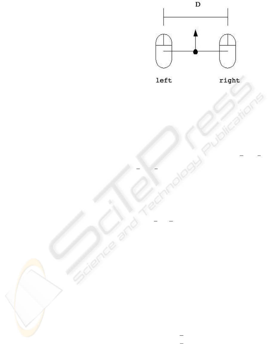
tion. For sake of ease, we place the mice at a certain

distance D, so that they are parallel between them and

orthogonal w.r.t. their joining line (see Figure 1). We

consider their mid-point as the position of the robot

and their direction (i.e., their longitudinal axis point-

ing toward their keys) as its orientation.

Each mouse measures its movement along its hori-

zontal and vertical axes. We hypothesize that, during

the sampling period (discussed in Section 4), the robot

Figure 1: The relative positioning of the two mice

moves with constant tangential and rotational speeds.

This implies that the robot movement can be approx-

imated by an arc of circumference. So, we have to

estimate the 3 parameters that describe the arc of cir-

cumference (i.e., the (x,y)-coordinates of the center

of the circumference and the arc angle), given the 4

readings taken from the two mice. We call x

and y

the measures taken by the mouse on the right, while

and y

are those taken by the mouse on the left.

Actually, we have only 3 independent data; in fact,

we have the constraint that the respective position of

the two mice cannot change. This means that the mice

should read always the same displacement along the

line that joins the centers of the two sensors. So, if

we place the mice as in Figure 1, we have that the

x-values measured by the two mice should be always

equal: x

= x

. In this way, we can compute how

much the robot pose has changed in terms of ∆x, ∆y,

and ∆θ.

If the robot makes an arc of circumference, it can

be shown that also each mouse will make an arc of cir-

cumference, which is characterized by the same cen-

ter and the same arc angle (but with a different radius).

During the sampling time, the angle α between the x-

axis of the mouse and the tangent to its trajectory does

not change. This implies that, when a mouse moves

along an arc of length l, it measures always the same

values independently from the radius of the arc (see

Figure 2). So, considering an arc with an inﬁnite ra-

dius (i.e., a segment), we can write the following re-

lations:

x = l cos(α) (1)

y = l sin(α). (2)

From Equations 1 and 2, we can compute both the

angle between the x-axis of the mouse and the tangent

to the arc:

ICINCO 2004 - ROBOTICS AND AUTOMATION

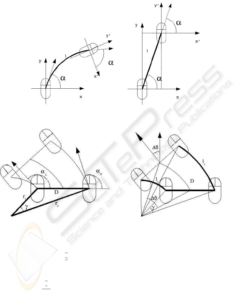
Figure 2: Two different paths in which the mouse readings are the same

Figure 3: The triangle made up of the joining lines and the

two radii

α = arctan

, (3)

and the length of the covered arc:

l =

x|, α = 0, π

sin α

, otherwise

(4)

In order to compute the orientation variation we ap-

ply the theorem of Carnot to the triangle made by the

joining line between the two mice and the two radii

between the mice and the center of their arcs (see Fig-

ure 3):

Figure 4: The angle arc of each mouse is equal to the change

in the orientation of the robot

= r

+ r

− 2 cos(γ)r

, (5)

where r

and r

are the radii related to the arc of cir-

cumferences described respectively by the mouse on

the right and the mouse on the left, while γ is the an-

gle between r

and r

. It is easy to show that γ can be

computed by the absolute value of the difference be-

tween α

and α

(which can be obtained by the mouse

measures using Equation 3): γ = |α

− α

The radius r of an arc of circumference can be com-

puted by the ratio between the arc length l and the arc

angle θ. In our case, the two mice are associated to

arcs under the same angle, which corresponds to the

change in the orientation made by the robot, i.e. ∆θ

DEAD RECKONING FOR MOBILE ROBOTS USING TWO OPTICAL MICE

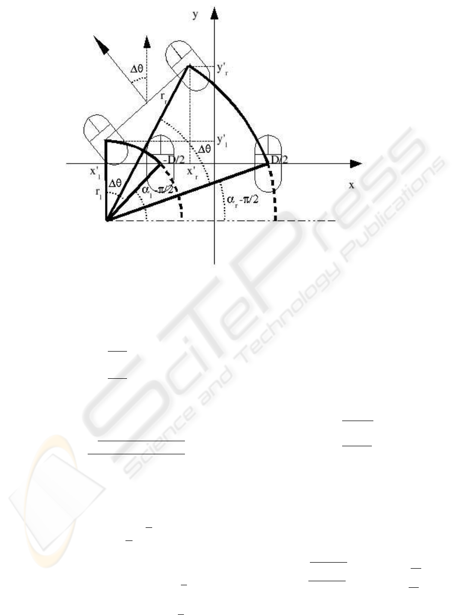
Figure 5: The movement made by each mouse

(see Figure 4). It follows that:

|∆θ|

(6)

|∆θ|

. (7)

If we substitute Equations 6 and 7 into Equation 5,

we can obtain the following expression for the orien-

tation variation:

∆θ = sign(y

− y

)

+ l

− 2 cos(γ)l

(8)

The movement along the x and y-axes can be de-

rived by considering the new positions reached by the

mice (w.r.t. the reference system centered in the old

robot position) and then computing the coordinates of

their mid-point (see Figure 5). The mouse on the left

starts from the point of coordinates (-

;0), while the

mouse on the right starts from (

;0). The formulas

for computing their coordinates at the end of the sam-

pling period are the following:

= r

(sin (α

+ ∆θ) − sin (α

)) sign(∆θ) +

(9)

= r

(cos (α

) − cos (α

+ ∆θ)) sign(∆θ) (10)

= r

(sin (α

+ ∆θ) − sin (α

)) sign(∆θ) −

(11)

= r

(cos (α

) − cos (α

+ ∆θ)) sign(∆θ). (12)

From the mice positions, we can compute the

movement executed by the robot during the sampling

time with respect to the reference system centered in

the old pose using the following formulas:

∆x =

+ x

(13)

∆y =

+ y

. (14)

The absolute coordinates of the robot pose at time

t + 1 (X

t+1

, Y

t+1

, Θ

t+1

) can be compute by know-

ing the absolute coordinates at time t and the rela-

tive movement carried out during the period (t; t + 1]

(∆x, ∆y, ∆θ) through these equations:

t+1

= X

∆x

+ ∆y

cos

+ arctan

∆y

∆x

¶¶

(15)

t+1

= Y

∆x

+ ∆y

sin

+ arctan

∆y

∆x

¶¶

(16)

t+1

= Θ

+ ∆θ. (17)

ICINCO 2004 - ROBOTICS AND AUTOMATION

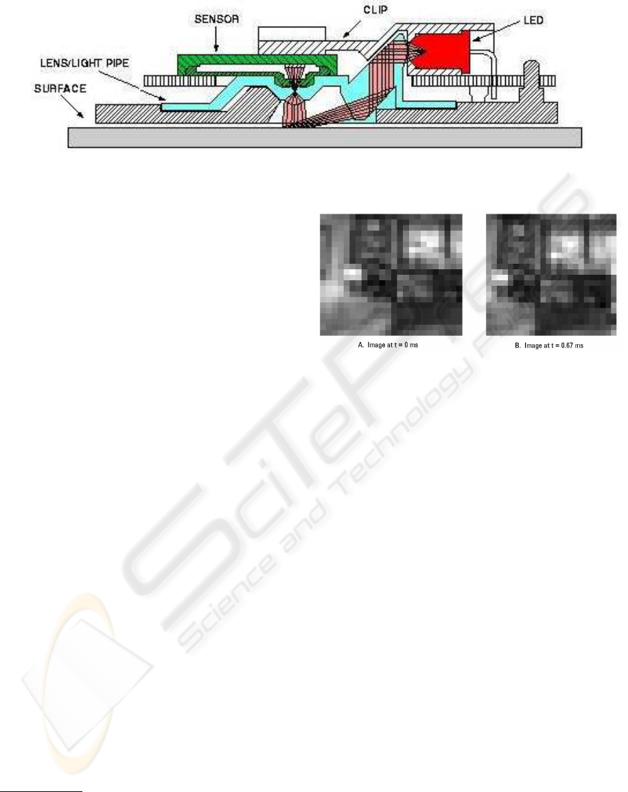
Figure 6: The schematic of an optical mouse

4 MICE CHARACTERISTICS

AND SYSTEM

PERFORMANCES

The performance of the odometry system we have de-

scribed depends on the characteristics of the solid-

state optical mouse sensor used to detect the dis-

placement of the mice. Commercial optical mice use

the Agilent ADNS-2051 sensor (Agilent Technolo-

gies Semiconductor Products Group, 2001) a low cost

integrated device which measures changes in posi-

tion by optically acquiring sequential surface images

(frames hereafter) and determining the direction and

magnitude of movement.

The main advantage of this sensor with respect to

traditional mechanical systems for movement detec-

tion is the absence of moving parts that could be dam-

aged by use or dust. Moreover it is not needed a

mechanical coupling of the sensor and the ﬂoor thus

allowing the detection of movement in case of slip-

ping and on many surfaces, including soft, glassy, and

curved pavements.

4.1 Sensor Characteristics

The ADNS-2051 sensor is essentially a tiny, high-

speed video camera coupled with an image proces-

sor, and a quadrature output converter (Agilent Tech-

nologies Semiconductor Products Group, 2003). As

schematically shown in Figure 6

, a light-emitting

diode (LED) illuminates the surface underneath the

sensorreﬂecting off microscopic textural features in

the area. A plastic lens collects the reﬂected light and

forms an image on a sensor. If you were to look at the

image, it would be a black-and-white picture of a tiny

section of the surface as the ones in Figure 7. The sen-

sor continuously takes pictures as the mouse moves at

Images reported in Figure 6, 7 and 8 are taken

from (Agilent Technologies Semiconductor Products

Group, 2001) and (Agilent Technologies Semiconductor

Products Group, 2003) and are copyright of Agilent Tech-

nologies Inc.

Figure 7: Two simple images taken from the mice. Beside

the noise you can notice the displacement of the pixels in

the images from right to left and top to bottom.

1500 frames per second or more, fast enough so that

sequential pictures overlap. The images are then sent

to the optical navigation engine for processing.

The optical navigation engine in the ADNS-2051

identiﬁes texture or other features in the pictures and

tracks their motion. Figure 7 illustrates how this is

done by showing two images sequentially captured as

the mouse was panned to the right and upwards; much

of the same “visual material” can be recognized in

both frames. Through an Agilent proprietary image-

processing algorithm, the sensor identiﬁes common

features between these two frames and determines the

distance between them; this information is then trans-

lated into ∆x and ∆y values to indicate the sensor

displacement.

By looking at the sensor characteristics, available

through the data sheet, it is possible to estimate

the precision of the measurement and the maximum

working speed of the device. The Agilent ADNS-

2051 sensor is programmable to give mouse builders

(this is the primary use of the device) 400 or 800 cpi

resolution, a motion rate of 14 inches per second, and

frame rates up to 2,300 frames per second. At recom-

mended operating conditions this allows a maximum

operating speed of 0.355 m/s with a maximum ac-

celeration of 1.47 m/s

These values are mostly due to the mouse sensor

(i.e., optical vs. mechanical) and the protocol used to

DEAD RECKONING FOR MOBILE ROBOTS USING TWO OPTICAL MICE

transmit the data to the computer. According to the

original PS/2 protocol, still used in mechanical de-

vices featuring a PS/2 connector, the ∆x and ∆y dis-

placements are reported using 9 bits (i.e., 1 byte plus

a sign bit) espressing values in the range from −255 to

+255. In these kind of mouse resolution can be set to

1, 2, 4, or 8 counts per mm and the sample rate can be

10, 20, 40, 60, 80, 100, and 200 samples per second.

The maximum speed allowed not to have an overﬂow

of the mouse internal counters is obtained by reducing

the resolution and increasing the sample rate. How-

ever, in modern mice with optical sensor and USB in-

terface these values are quite different, in fact the USB

standard for human computer interface (USB Imple-

menter’s Forum, 2001) restricts the range for ∆x and

∆y displacements to values from −128 to +127 and

the sample rate measured for a mouse featuring the

ADNS-2051 is 125 samples per second.

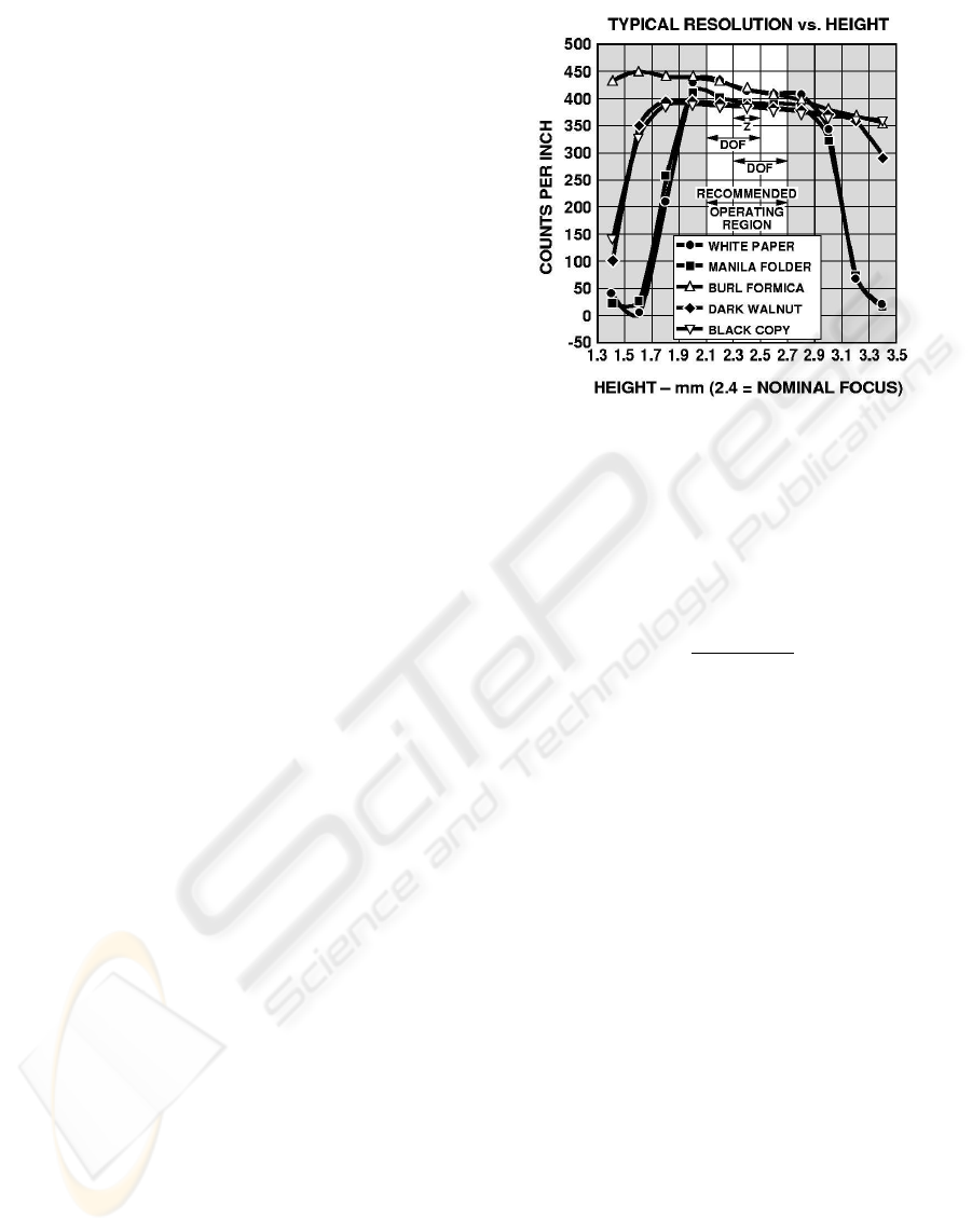
4.2 Mice Calibration Process

The numbers we have reported in the previous subsec-

tion reﬂect only nominal values for the sensor char-

acteristics since its resolution can vary depending on

the surface material and the height of the sensor from

the ﬂoor as described in Figure 8. This variation in

sensor readings calls for an accurate mounting on the

robot and a minimal calibration procedure before ap-

plying the formulas described in the previous section

in order to reduce systematic errors in odometry. In

fact systematic errors in odometry are often due to a

wrong assumptions on the model parameters and they

can be signiﬁcantly reduced by experimental estima-

tion of right values. Our model systematic errors are

mostly due to the distance D between the mice and

the exact resolution of the sensors. To estimate the

last parameter, we have moved 10 times the mice on a

20 cm straight track and estimated in 17.73 the num-

ber of ticks per mm (i.e., 450 cpi) through the aver-

age counts for the mice ∆y displacements.

The estimation of the distance between the two

mice has been calibrated after resolution calibration

by using a different procedure. We rotated the two

mouse around their middle point for a ﬁxed angle η

(π/2 rad in our experiments) and we measured again

their ∆y displacements. These two measures have to

be equal to assure we are rotating around the real mid-

dle point and the ∆x displacement should be equal to

zero when the mice are perpendicular to the radius.

Provided the last two constraints we can estimate their

distance according to the simple formula

D = ∆y/η. (18)

However, it is not necessary to rotate the mice

around their exact middle point, we can still estimate

their distance by rotating them around a ﬁxed point

Figure 8: Typical resolution vs. Z (distance from lens refer-

ence plane to surface) for different surfaces

on the joining line and measuring the ∆y

and ∆y

Given these two measurements we can compute D by

using

D =

∆y

+ ∆y

. (19)

5 EXPERIMENTAL RESULTS

In order to validate our approach, we take two USB

optical mice featuring the Agilent ADNS-2051 sen-

sor, which can be commonly purchased in any com-

mercial store. We ﬁx them as described in Section 3,

taking care of making them stay in contact with the

ground. We made our experiments on a carpet, like

those used in the RoboCup Middle Size League us-

ing the recommended operating setting for the sensor

(i.e., nominally 400 cpi at 1500 frames per second)

and calibrating the resolution to 450 cpi and the dis-

tance D between the mice to 270 mm with the pro-

cedure previously described.

The preliminary test we made is the UMBmark

test, which was presented by (Borenstein and Feng,

1994). The UMBmark procedure consists of measur-

ing the absolute actual position of the robot in or-

der to initialize the on-board dead reckoning start-

ing position. Then, we make the robot travel along

a 4x4 m square in the following way: the robot stops

after each 4m straight leg and then it makes a 90

turn on the spot. When the robot reaches the starting

area, we measure its absolute position and orientation

and compare them to the position and orientation cal-

culated by the dead reckoning system. We repeated

ICINCO 2004 - ROBOTICS AND AUTOMATION

this procedure ﬁve times in clockwise direction and

ﬁve times in counter-clockwise. The measure of dead

reckoning accuracy for systematic errors that we ob-

tained is E

max,syst

= 114 mm, which is compara-

ble with those achieved by other dead reckoning sys-

tems (Borenstein and Feng, 1996).

6 RELATED WORKS

As we said in Section 1, Mobile Robot Position-

ing has been one of the ﬁrst problem in Robotics

and odometry is the most widely used navigation

method for mobile robot positioning. Classical odom-

etry methods based on dead reckoning are inexpen-

sive and allow very high sample rates providing good

short-term accuracy. Despite its limitations, many re-

searcher agree that odometry is an important part of

a robot navigation system and that navigation tasks

will be simpliﬁed if odometric accuracy could be im-

proved.

The fundamental idea of dead reckoning is the inte-

gration of incremental motion information over time,

which leads inevitably to the unbounded accumula-

tion of errors. Speciﬁcally, orientation errors will

cause large lateral position errors, which increase pro-

portionally with the distance traveled by the robot.

There have been a lot of work in this ﬁeld especially

for differential drive kinematics and for systematic er-

ror measurement, comparison and correction (Boren-

stein and Feng, 1996).

First works in odometry error correction were

done by using and external compliant linkage vehicle

pulled by the mobile robot. Being pulled this vehicle

does not suffer from slipping and the measurement

of its displacing can be used to correct pulling robot

odometry (Borenstein, 1995). In (Borenstein and

Feng, 1996) the authors propose a practical method

for reducing, in a typical differential drive mobile

robot, incremental odometry errors caused by kine-

matic imperfections of mobile encoders mounted onto

the two drive motors.

Little work has been done for different kinemat-

ics like the ones based on omnidirectional wheels. In

these cases, slipping is always present during the mo-

tion and classical shaft encoder measurement leads

to very large errors. In (Amini et al., 2003) the Per-

sia RoboCup team proposes a new odometric system

which was employed on their full omni-directional

robots. In order to reduce non-systematic errors,

like those due to slippage during acceleration, they

separate odometry sensors from the driving wheels.

In particular, they have used three omni-directional

wheels coupled with shaft encoders placed 60

apart

of the main driving wheels. The odometric wheels are

connected to the robot body through a ﬂexible struc-

ture in order to minimize the slippage and to obtain a

ﬁrm contact of the wheels with the ground. Also this

approach is independent from the kinematics of the

robot, but its realization is quite difﬁcult and, how-

ever, it is affected by (small) slippage problems.

An optical mouse was used in the localization sys-

tem presented in (Santos et al., 2002). In their ap-

proach, the robot is equipped with an analogue com-

pass and an optical odometer made out from a com-

mercially available mouse. The position is obtained

by combining the linear distance covered by the robot,

read from the odometer, with the respective instanta-

neous orientation, read from the compass. The main

drawback of this system is due to the low accuracy of

the compass which results in systematic errors.

However, odometry is inevitably affected by the

unbounded accumulation of errors. In particular, ori-

entation errors will cause large position errors, which

increase proportionally with the distance travelled by

the robot. There are several works that propose meth-

ods for fusing odometric data with absolute position

measurements to obtain more reliable position esti-

mation (Cox, 1991; Chenavier and Crowley, 1992).

7 CONCLUSIONS

We have presented a dead reckoning sensor based on

a pair of optical mice. The main advantages are good

performances w.r.t. the two main problems that affect

dead reckoning sensors: slipping and crawling. On

the other hand, this odometric system needs that the

robot operates on a ground with a surface on which

the mice always read with the same resolution.

Due to its characteristics, the proposed sensor can

be successfully applied with many different robot ar-

chitectures, being completely independent from the

speciﬁc kinematics. In particular, we have developed

it for our omnidirectional Robocup robots, which will

be presented at Robocup 2004.

REFERENCES

Agilent Technologies Semiconductor Products Group

(2001). Optical mice and hiw they work: The optical

mouse is a complete imaging system in a tiny pack-

age. Technical Report 5988-4554EN, Agilent Tech-

nologies Inc.

Agilent Technologies Semiconductor Products Group

(2003). Agilent adns-2051 optical mouse sesor data

sheet. Technical Report 5988-8577EN, Agilent Tech-

nologies Inc.

Amini, P., Panah, M. D., and Moballegh, H. (2003). A new

odometry system to reduce asymmetric errors for om-

DEAD RECKONING FOR MOBILE ROBOTS USING TWO OPTICAL MICE

nidirectional mobile robots. In RoboCup 2003: Robot

Soccer World Cup VII.

Borenstein, J. (1995). Internal correction of dead-reckoning

errors with the compliant linkage vehicle. Journal of

Robotic Systems, 12(4):257–273.

Borenstein, J. and Feng, L. (1994). UMBmark - a

method for measuring, comparing, and correcting

dead-reckoning errors in mobile robots. In Proceed-

ings of SPIE Conference on Mobile Robots, Philadel-

phia.

Borenstein, J. and Feng, L. (1996). Measurement and

correction od systematic odometry errors in mobile

robots. IEEE Transactions on Robotics and Automa-

tion, 12(6):869–880.

Chenavier, F. and Crowley, J. (1992). Position estima-

tion for a mobile robot using vision and odometry.

In Proceedings of IEEE International Conference on

Robotics and Automation, pages 2588–2593, Nice,

France.

Cox, I. (1991). Blanche - an experiment in guidance and

navigation of an autonomous mobile robot. IEEE

Transactions on Robotics and Automation, 7(3):193–

204.

Santos, F. M., Silva, V. F., and Almeida, L. M. (2002). A

robust self-localization system for a small mobile au-

tonomous robot. In Preceedings of ISRA.

USB Implementer’s Forum (2001). Universal serial bus:

Device class deﬁnition for human interface devices.

Technical Report 1.11, USB.

ICINCO 2004 - ROBOTICS AND AUTOMATION