AUTOLOCALIZATION USING THE CONVOLUTION OF THE
EXTENDED ROBOT
Eduardo Espino
Univ. of Salamanca. - Spain.
Vidal Moreno
Univ. of Salamanca - Spain.
Belen Curto
Univ. of Salamanca - Spain.
Ramiro Aguilar
Univ. of Salamanca. - Spain.
Keywords:
Autolocalization, Convolution, Extended mobile Robot
Abstract:
In order to construct autonomous robots which they move in a indoor environment, it is necessary to solve
several problems such as the autolocalization. The problem of the autolocalization in a robot mobile consists
of it must find its location within an apriori known map of its surroundings using the perceived distances by
its sensors. The difficulties come from the fact that the signals of the sensors have noise, as well as the control
signals and also the map could differ from the reality of the surroundings.
The method which we presented joins the measures of the sensors and the signals of control in the called map
of the extended robot; through of the convolution of this map and the a priori map of the environment, we can
find the best matching between them, after a search into this calculated values, the location is obtained as a
configuration that corresponds to the global maximum convolution.
The method was implemented in an sonar-based robot, with kinematics differential. The results have validated
widely our proposal.
1 INTRODUCTION
During the last years, mobile robots have been
thought to perform task in an autonomous way or
work at high risk environment. In this way, the autolo-
calization is considered as one of the most important
ability to be implemented.
Ones developed works to solve the autolocation,
are based in probabilistic filters; the most referenced
author is Kalman(Bar-Shalom and Li, 1995). Al-
though one of its main problems is that the signals
caught by the sensors differ from a signal with Gaus-
sian error.
In additional, the Monte Carlo algorithm (S. Turn
and Dellaer, 2000) recalculate the new hypothetical
states of the position of robot according to the ac-
tion model (kinematics). Between the disadvantages
of the probabilistics methods it is that could not con-
verge to the right solution if the generated hypotheses
were not near enough of it.
Many researchers use the icon-based loca-
tion(G. Schaffer and Stentz, 1992) where the caught
information of the surroundings is plotted on a map
that is matched with the a priori map of the environ-
ment, based on the minimal distance. The position
of the robot is obtained so that the error between the
distance of the landmarks is the smallest. A similar
approach is the matched based on grid maps (Schiele
and Crowley, 1994), the first grid map, centered in the
robot and modeling its local environment using the
last readings of the sensors, and the second grid map
is a global model of the environment. A correlation
index is increased when the grids are in the same state
and diminishes when they have different states. At
the end, with the maximum in the correlation index
is the transformation that generates the maximum
index, so that we obtain the correspondence between
the local and the global map. Until now the matched
problem grid to grid has been the processing time
due to the high computacional load. The method
presented here, perform the matching between the
first map of the robot including the readings of the
sensors and the second a piori map of the environment
through a convolution. We can find the best matching
between them, after a search into this calculated
values, the location is obtained as a configuration
that corresponds to the global maximum convolution.
Using the fast Fourier transformed diminishing the
365
Espino E., Moreno V., Curto B. and Aguilar R. (2004).
AUTOLOCALIZATION USING THE CONVOLUTION OF THE EXTENDED ROBOT.
In Proceedings of the First International Conference on Informatics in Control, Automation and Robotics, pages 365-369
DOI: 10.5220/0001143203650369
Copyright
c
 SciTePress

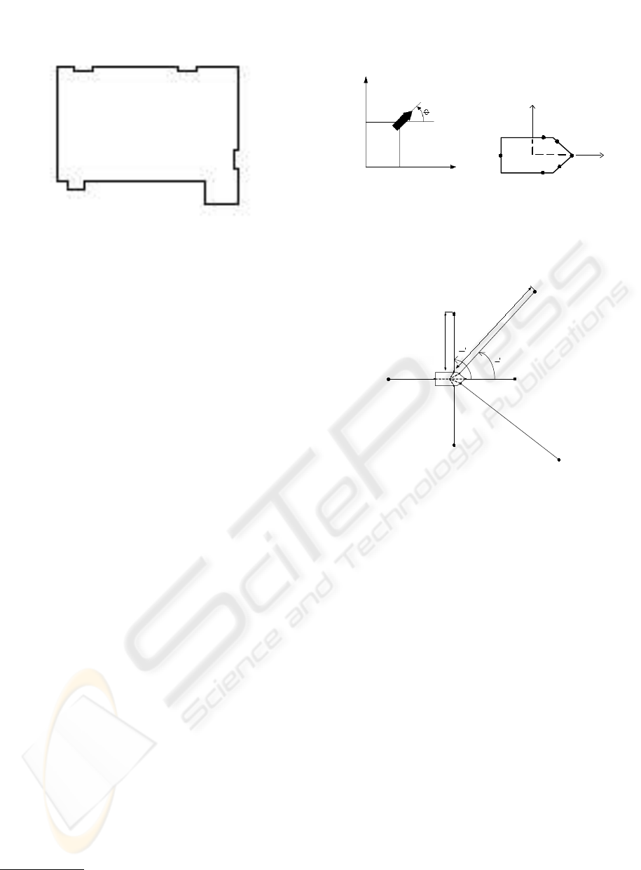
Figure 1: Map of the environment W in a matrix of
128X128 pixels.
computacional load significantly. In the section 2 we
describe process of matching the environment map
and the extended robot map, in section 3 we present
some improvenment to the method and in section 4
we present results and conclusions of our work.
2 MATCHING THE
ENVIRONMENT AND THE
EXTENDED ROBOT MAPS
2.1 The environment map
The a priori map is a matrix (W), where the obstacles
or the walls
1
are ones and the free place are zeros (fig
1).
w(x, y) =
½
1 (x, y) ∈ Obstacle
0 (x, y) /∈ Obstacle
(1)
2.2 The extended robot
With the readings of the robot’s sensors we can built
a map of the position of the obstacles, which we will
call the extended robot.
The initial representation of the robot P
0
is de-
termined by a set of points that in this case could
be enough to consider only the locations of the sen-
sors (s elements), because they are in contour of
the mobile robot (fig. 2b). Therefore the vector of
representative points of the robot P
0
has s elements
[p
0,0
, ..., p
s−1,0
]
T
referred to a local coordinates sys-
tem
2
.
We define as extended robot to the composition of
the robot’s point defined by the representative points
1
In general, word obstacle will include walls too.
2
The center of the robot, the midpoint of the segment
that links the two driving wheels, is placed in the coordi-
nates (0,0) and the axis x oriented to the frontal part of the
robot.
X
G
Y
G
x
y
(a)
Y
L
X
L
p
1,0
p
0,0
p
2,0
p
3,0
p
4,0
p
5,0
cg
(b)
Figure 2: (a) The configuration q is given by three elements
x, y y θ. (b) Representative points of the robot P
0
for a
configuration q
0
.
l
0
0
0
1
pe
0,0
pe
1,0
pe
2,0
pe
3,0
pe
4,0
pe
5,0
p
o
p
1
1,0
l
0,0
Figure 3: Distances Captured by the Robot
(p
i,0
∈ P
0
) whith the distances (l
i,0
∈ L
0
) captured by
the sensors in its direction θ
0
i
in the local coordinates
system (figure 3).
The vector of Points of the extended Robot PE
0
([pe
0,0
, ...pe
s−1,0
]
T
) is calculated of the following
way:
PE
0
= P
0
+ L
0





cosθ
0
0
senθ
0
0
... ...
cosθ
0
i
senθ
0
i
... ...
cosθ
0
s−1
senθ
0
s−1





(2)
Finally we can build the Extended Robot Map A
0
like a matrix which size is N X N (fig. 4) and it is
obtained using the PE
0
vector, of the following way:
a
0
(x, y) =
½
1 (x, y) ∈ PE
0
0 (x, y) /∈ PE
0
(3)
As in the location problem we don’t know the an-
gle of the robot, we could find one extended robot for
each possible orientation of the robot. The considered
angles are θ
k
= k.2π/N where k : 0, 1, ..., (N − 1)
and N is the number of possible orientations in the
discrete space. Then we must rotate the coordinates
ICINCO 2004 - ROBOTICS AND AUTOMATION
366

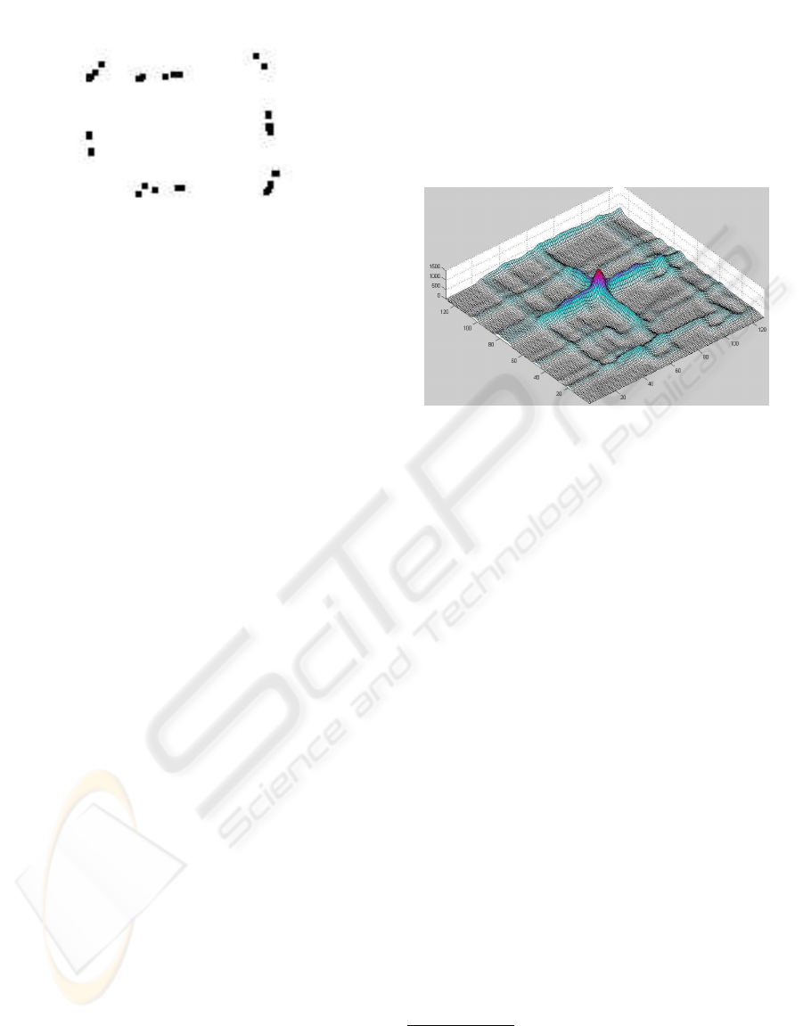
Figure 4: The extended Robot Map (A
0
) in a matrix of
128X128 pixels..
of PE
0
to obtain a new vector of representative points
of the extended robot, according to the following re-
lation:
R(θ
k
) =
·
cosθ
k
senθ
k
−senθ
k
cosθ
k
¸
(4)
PE
k
= PE
0
. R(θ
k
) (5)
The matrix of the extended robot in a θ
k
orientation
is calculate as the equation 3 in the following form:
a
k
(x, y) =
½
1 (x, y) ∈ PE
k
0 (x, y) /∈ PE
k
(6)
2.3 Matching Maps by Convolution
The matching between the environment and each ex-
tended robot maps is performed using a measure-
ments of similarities based in the convolution of
maps.
Each point of the extended robot vector has a bit
of information about position of obstacles in the envi-
ronment, so we can find point of similarities between
the robot extended map (A
k
) and the map of the envi-
ronment (W). The grade of similarity can be estimate
putting each map of the extended robot over the map
of the environment, in this position, we can calculate
the addition of products of each pixel of the extended
robot with the under pixcel of the environment.
c
k
(0, 0) =
X
i=N−1
i=0
X
j=N−1
j=0
w(i, j).a
k
(i, j) (7)
A new value can be calculate if the extended robot
map is moved to a new (x, y) position over the envi-
ronment map.
c
k
(x, y) =
X
i=N−1
i=0
X
j=N−1
j=0
w(i, j).a
k
(i−x, j−y)
(8)
Using a change of variables we define a new matrix
A’
k
where :
a’
k
(x, y) = a
k
(−x, −y) (9)
So that the equation 8 in matricial form result in:
C
k
= A’
k
⊗ W (10)
Where ⊗ is the convolution 2-dimensional
3
.
Figure 5: The Convolution Matrix C
0
.
Figure 5 show the convolution matrix C
k
for A
0
and W. We can see a local maximum value the near to
the center of the matrix.
The greater value of c
k
(x,y), the greater similarity
between maps, so we think that the global maximum
value in C
k
(k : 0, .., N − 1) given us the position
(x, y, θ
k
) of the extended robot refered to the envi-
ronment map.
As the C matrix is calculated by layers (C
k
), the
process is repeated N times. In C, we will do a search
for the configurations ˆq that satisfies the condition
C(ˆq) = max(C) (11)
This configuration will be the location of the
robot
4
.
If we considered the maps W and A
k
as square ma-
trixs N dimensional, the time required for the calcu-
lation of C
k
in 2D is O(N
2
logN) and in addition, we
must consider N possible directions, reason why, the
operation must be repeated N times, thus, the time
required to calculate C is O(N
3
logN).
3 IMPROVING THE METHOD
To implement the method exposed in subsection
2.3 was necesary to make variations that assure the
3
The procedure for the fast calculation of the C matrix
(Kavraki, 1995), using the discrete Fourier transformed, is
C
k
= DFT
−1
(DFT (A’
k
) × DFT (W)).
4
The search is performed varying x from 0 to (N − 1),
y from 0 to (N − 1) and θ from 0 to (2π ∗ (N − 1)/N)
AUTOLOCALIZATION USING THE CONVOLUTION OF THE EXTENDED ROBOT
367

unique solution, due to there could be more than one
configuration ˆq. We found that the method is lacking
in:
• Insufficient information to detect asymmetries and
the limits of the environment.
• No consider no-Gaussian Error information of sen-
sors.
• No consider Gaussian Error information of envi-
ronment map and sensors
So we propose in 3.1, 3.2 and 3.3 some operations
to overcome those problems.
3.1 Increasing the number of points
in PE vectors
To increase the number of points in PE vectors, we
chosed a specific exploration; the core is that the robot
must complete N small turns, until 2π radians. At
each position
5
q
j
, the robot takes readings from the
sensors (L
j
vector
6
) and with them, it can build the
extended robot (PEX
j
) respect to a local coordenate
system for the initial configuration q
0
by performing
a frame rotation.
PEX
j
=
Ã
P
0
+ L
j
.
"
... ...
cosθ
0
i
senθ
0
i
... ...
#!
.R(φ
j
)
(12)
Since, the N vectors of representative points
(PEX
0
, PEX
1
...PEX
N−1
) are referred to the same
coordinate system (refereed to q
0
) we can associate
them in a single vector, the new Total Vector of Points
of the Extended Robot (
~
PE
0
) with length s.N , which
contains the coordinates of the end of points for all
extended robots generated.
~
PE
0
=





~pe
0,0
...
~pe
sj+i,0
...
~pe
s.N−1,0





=





pex
0,0
...
pex
i,j
...
pex
s−1,N−1





(13)
This exploration has the additional advantage that
the final configuration q
N
of the robot is approxi-
mately equal to the initial configuration q
0
, so that if
our calculations are based on the initial configuration,
we will find the present configuration of the robot at
the moment of the calculation.
5
Applying the kinematics of the robot, the sequences of
configurations q
0
, q
1
... q
N−1
is invariant in two first ele-
ments x
j
and y
j
and only the third element, φ
j
, changes,
being φ
j
= j ∗ 2π/N. In addition q
0
is the configuration
0,0,0 and it is represented in the center of the A matrix
6
the matrix of distances L where each element l
i,j
cor-
responds to the reading of the sonar i in the configuration
q
j
.
3.2 Filtering the signals caught by
the sonars (L matrix)
In a real case, using the total vector of points
~
PE
0
to build the map of the extended robot, we obtained
a figure where it is not possible to find any similar-
ity between the environment map and the extended
robot, so the first conclusion is the errors are positive
generally or the measures captured by the sonars are
greater than the measures calculated by the model of
the environment.
We made a comparison of the measures captured by
the sonars with the theoretical values, calculated from
the model of the environment; for the theoretical val-
ues, we can observe 4 zones of local minima, also it
is possible to see the similarity between the theoret-
ical values and the caught ones by the sensors in the
zones of minimums. These zones of local minimums
correspond at the moments in which the sound waves
fall perpendicularly to the surface of obstacle. Conse-
quently we can conclude the readings closer to local
minimums, will be more reliable and we will accept
those values, discarding the other readings.
The filter algorithm for the length l
i,j
, is performed
by the following equation:
~
l
i,j
=
½
l
i,j
l
i,j
< l
i,j−1
AND l
i,j
< l
i,j+1
0 l
i,j
> l
i,j−1
OR l
i,j
> l
i,j+1
(14)
Now we can recalculate the PEX
j
matrix using the
new
~
L
j
matrix in the equation 12.
3.3 Rebuilding of the environment
map (W) and the extended robot
(A) maps.
To consider the inaccuracies in the process of build-
ing the map, we should to calculate the convolution
between the map and a mask, this mask matrix (e)
has the form like a probabilistic distribution. We use
the cosene function to approximate this probabilistic
distribution. The value of the central element is one,
the others elements have a value less thas one, in the
bounds of the mask matrix there are zeros values(fig
6).
~
W = W ⊗ e (15)
After the convolution, we obtein a new map of the
environment (
~
W), where there are greather values are
in the same place of the bitmap original, the lower
values are in the surroundings of the obstacles.
Similarly, we could consider the inaccuracies in the
extended robot maps, using the mask matrix (e).
~
A
k
= A
k
⊗ e (16)
ICINCO 2004 - ROBOTICS AND AUTOMATION
368

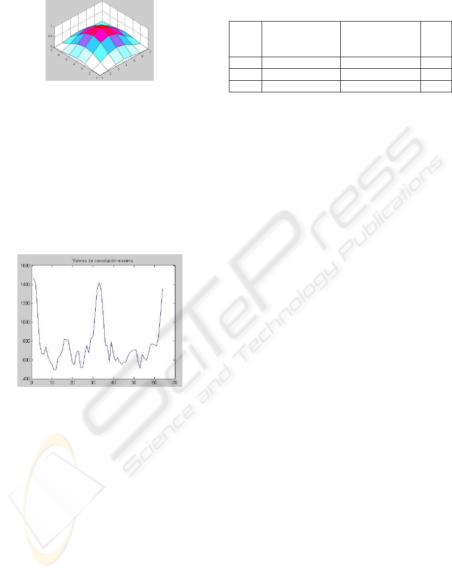
Figure 6: The mask matrix (e) of the probabilistic distribu-
tion with 7X7 elements
4 RESULTS AND CONCLUSIONS
In order to prove the validity of this procedures, it was
applied in an experimental robot AmigoBot devel-
oped by center SRI of Stanford. This robot, 8 sonars-
based, performs the exploration in sweeping type (32
rotations). We has been chosen to prove the method
in 3 locations different (real position) in a rectangle
room, which approx dimensions are 6 x 9 meters and
has asymmetries.
Figure 7: Local maxima values for each possible orienta-
cion θ
k
After calculating the Convolution C, we mark the
maximun value in each possible orientation and we
show it in the figure 7. The search of the q give us the
configuration ˆq which is the estimated position of the
robot, and it could be compared with the real position
in the Table 1. The range of errors is in decimeters,
and the resolution of the matrixes is one decimeter
for a information pixel, the dimension of the matrixes
was of 128 X 128, and the resulting C was of 128
X 128 X 64. If it is necessary greater resolution, the
dimension of the matrixes will be greater therefore the
time of calculation is increased.
4.1 Conclusions
The development of a tool for the automatic localiza-
tion of mobile robots, which navigate in structured en-
vironment, is the main target of this work.
Table 1: Results for the points of test A, B and C
point real position real estimate position error
of q
0
ˆq
0
test x, y, φ ˆx, ˆy,
ˆ
φ dm
A 47.10, 67.48, 0
0
46.68, 67.81, 0
0
0.53
B 62.11, 67.48, 0
0
59.97, 66.22, 0
0
2.48
C 77.05, 67.48, 0
0
74.83, 65.07, 0
0
3.27
The implementation only requires a bit map as a
model of the environment, without having limitation
for the shape or for the position between obstacles,
being able to deduce that the time of processing does
not depend on the complexity of the environment.
It is a global deterministic location, because, the
method verifies all the posible configurations. The fil-
ter of minimums rejects noisy readings therefore the
method is robust to great disturbances like in sonars.
The calculation of the Convolution is a low load in
the processor, thanks to the fast Fourier transformed
applied.
Finally the algorithm of autolocalizacin in an ex-
perimental robot has been implemented and it has
been possible to validate the results in real situations.
Therefore, the robot has been equipped of the capac-
ity to find its location, thus, it has greater autonomy.
REFERENCES
Bar-Shalom, Y. and Li, X. (1995). Multitarget-Multisensor
Tracking: Principles and Techniques. YBS ISBN 0-
9648312-0-1.
G. Schaffer, J. G. and Stentz, A. (1992). Comparison of two
range-based pose estimators for a mobile robot. In
Proceedings of the 1992 SPIE Conference on Mobile
Robots, pages 661–667, Boston.
Kavraki, L. E. (1995). Computation of configuration-space
obstacles using the fast fourier transform. IEEE Tr. on
Robotics and Automation, 11(3):408–413.
S. Turn, D. Fox, W. B. and Dellaer, F. (2000). Robust monte
carlo localization for mobile robots. Technical report,
Carnegie Mellon University.
Schiele, B. and Crowley, J. (1994). A comparison of po-
sition estimation techniques using occupancy grids.
In Proceedings of IEEE International Conference on
Robotics and Automation, pages 1628–1634, San
Diego, CA.
AUTOLOCALIZATION USING THE CONVOLUTION OF THE EXTENDED ROBOT
369