MOMENT-LINEAR STOCHASTIC SYSTEMS

Sandip Roy

Washington State University, Pullman, WA

George C. Verghese

Massachusetts Institute of Technology, Cambridge, MA

Bernard C. Lesieutre

Lawrence Berkeley National Laboratory, Berkeley, CA

Keywords:

jump-linear systems, linear state estimation and control, stochastic network models

Abstract:

We introduce a class of quasi-linear models for stochastic dynamics, called moment-linear stochastic systems

(MLSS). We formulate MLSS and analyze their dynamics, as well as discussing common stochastic models

that can be represented as MLSS. Further studies, including development of optimal estimators and controllers,

are summarized. We discuss the reformulation of a common stochastic hybrid system—the Markovian jump-

linear system (MJLS)—as an MLSS, and show that the MLSS formulation can be used to develop some

new analyses for MJLS. Finally, we brieﬂy discuss the use of MLSS in modeling certain stochastic network

dynamics. Our studies suggest that MLSS hold promise in providing a framework for modeling interesting

stochastic dynamics in a tractable manner.

1 INTRODUCTION

As critical networked infrastructures such as air trafﬁc

systems, electric power systems, and communication

networks have become more interdependent, the need

for models for large-scale and hybrid network dynam-

ics has grown. While the dramatic improvement in

computer processing speeds in recent years has some-

times facilitated predictive simulation of these net-

works’ dynamics, the development of models that al-

low not only prediction of dynamics but also network

control and design remains a challenge in several ap-

plication areas (see, e.g., (Bose, 2003)). In this article,

we introduce and give the basic analysis for a class

of models called moment-linear stochastic systems

(MLSS) that can represent some interesting stochas-

tic and hybrid system/network dynamics, and yet

are sufﬁciently structured to allow computationally-

attractive analyses of dynamics, state estimation, and

control. Our studies suggest that MLSS hold promise

as a modeling tool for a variety of stochastic and

hybrid dynamics, especially because they provide a

framework for several common stochastic and/or hy-

brid models in the literature, and because they can

capture some network dynamics in a tractable man-

ner.

Our research is partially concerned with hybrid

(mixed continuous- and discrete-state) dynamics.

Stochastic hybrid models whose dynamics are con-

strained to Markovian switching between a ﬁnite

number of linear time-invariant models have been

studied in detail, under several names (e.g., Marko-

vian jump-linear systems (MJLS) and linear jump-

Markov systems) (Loparo et al., 1991; Mazor et al.,

1998). Techniques for analyzing the dynamics of

MJLS, and for developing estimators and controllers,

are well-known (e.g., (Fang and Loparo, 2002; Costa,

1994; Mazor et al., 1998)). Of particular interest to us,

a linear minimum-mean-square error (LMMSE) esti-

mator for the continuous state of an MJLS was devel-

oped by (Costa, 1994), and quadratic controllers have

been developed by, e.g., (Chizeck and Ji, 1988). We

will show that similar estimation and control analyses

can be developed for MLSS, and hence can be applied

to a wider range of stochastic dynamics.

We are also interested in modeling stochastic net-

work interactions. There is wide literature on stochas-

tic network models that is largely beyond the scope of

this article. Of particular interest to us, several mod-

els from the literature on queueing and stochastic au-

tomata can be viewed as stochastic hybrid networks

(see (Kelly, 1979; Rothman and Zaleski, 1997; Dur-

rett, 1981) for a few examples). By and large, the

aims of the analyses for these models differ from our

aims, in that transient dynamics are not characterized,

and estimators and controllers are not developed. One

190

Roy S., Verghese G. and Lesieutre B. (2004).

MOMENT-LINEAR STOCHASTIC SYSTEMS.

In Proceedings of the First International Conference on Informatics in Control, Automation and Robotics, pages 190-197

DOI: 10.5220/0001143401900197

 SciTePress

class of stochastic automata of particular interest to

us are Hybrid Bayesian Networks (e.g., (Heskes and

Zoeter, 2003)). These are graphical models (i.e., mod-

els in which stochastic interactions are speciﬁed using

edges on a graph) with hybrid (i.e., mixed continuous-

state and discrete-state) nodal variables. Dynamic

analysis, inference (estimation), and parameter learn-

ing have been considered for such networks, but com-

putationally feasible methods are approximate.

We observe that stochastic systems models with

certain linear or quasi-linear structures (e.g., linear

systems driven by additive white Gaussian noise,

MJLS) are often widely tractable: statistics of tran-

sient dynamics can be analyzed, and LMMSE esti-

mators and optimal quadratic controllers can be con-

structed. Several stochastic network models with

quasi-linear interaction structures have also been

proposed—examples include the voter model or inva-

sion process (Durrett, 1981), and our inﬂuence model

(Asavathiratham, 2000). For these network models,

the quasi-linear structure permits partial characteriza-

tion of state occupancy probabilities using low-order

recursions. In this article, we view these various lin-

ear and quasi-linear models as examples of moment-

linear models—i.e., models in which successive mo-

ments of the state at particular times can be inferred

from equal and lower moments at previous times us-

ing linear recursions. This common representation

for quasi-linear system and network dynamics moti-

vates our formulation of MLSS, which are similarly

tractable to the examples listed above. The MLSS

formulation is further useful, in that it suggests some

new analyses for particular examples and elucidates

some other types of stochastic interactions that can be

tractably modeled.

The remainder of the article is organized as fol-

lows: in Section 2, we describe the formulation and

basic analysis—namely, the recursive computation of

state statistics—of MLSS. We also list common mod-

els, and types of stochastic interactions, that can be

captured using MLSS. Section 3 contains a summary

of further results on MLSS. In Section 4, we refor-

mulate the MJLS as an MLSS, and apply the MLSS

analyses to this model. We also list other common hy-

brid models that can be modeled as MLSS. Section 5

summarizes our studies on using MLSS to model net-

work dynamics. In this context, a discrete-time ﬂow

network model is developed in some detail.

2 MLSS: FORMULATION AND

BASIC ANALYSIS

An MLSS is a discrete-time Markov model in which

the conditional distribution for the next state given

the current state is specially constrained at each time-

step. These conditional distributions are constrained

so that successive moments and cross-moments of

state variables at each time-step can be found as lin-

ear functions of equal and lower moments and cross-

moments of state variables at the previous time-step,

and hence can be found recursively.

Formally, consider a discrete-time Markov process

with an m-component real state vector. The state (i.e.,

state vector) of the process at time k is denoted by

s[k]. We write {s[k]} to represent the state sequence

s[0], s[1], . . . and s

[k] to denote the ith element of

the state vector at time k. We stress that we do not

in general enforce any structure on the state variables,

other than that they be real; the state vector may be

continuous-valued, discrete-valued, or hybrid.

For this Markov process, we consider the con-

ditional expectation E(s[k + 1]

⊗r

| s[k]), for r =

1, 2, . . ., where the notation s[k + 1]

⊗r

refers to the

Kronecker product of the vector s[k + 1] with it-

self r times and is termed the rth-order state vec-

tor at time k. This expectation vector contains all

rth moments and cross-moments of the state variables

[k + 1], . . . , s

[k + 1] given s[k], and so we call the

vector the conditional rth (vector) moment for s[k+1]

given s[k]. We say that the process {s[k]} is rth-

moment linear at time k if the conditional rth moment

for s[k + 1] given s[k] can be written as follows:

E(s[k + 1]

⊗r

| s[k]) = H

r,0

[k] +

i=1

r,i

[k]s[k]

⊗i

(1)

for some set of matrices H

r,0

[k], . . . , H

r,r

[k].

The Markov process {s[k]} is called a moment-

linear stochastic system (MLSS) of degree br if it is

rth-moment linear for all r ≤ br, and for all times

k. If a Markov model is moment linear for all r and

k, we simply call the model an MLSS. We call the

constraint (1) the rth-moment linearity condition at

time k, and call the matrices H

r,0

[k], . . . , H

r,r

[k] the

rth-moment recursion matrices at time k. These re-

cursion matrices feature prominently in our analysis

of the temporal evolution of MLSS.

MLSS are amenable to analysis, in that we can ﬁnd

statistics of the state s[k] (i.e., moments and cross-

moments of state variables) using linear recursions.

In particular, for an MLSS of degree br, E(s[k + 1]

⊗r

)

(called the rth moment of s[k + 1]) can be found in

terms of the ﬁrst r moments of s[k] for any r ≤ br. To

ﬁnd these rth moments, we use the law of iterated ex-

pectations and then invoke the rth-moment linearity

MOMENT-LINEAR STOCHASTIC SYSTEMS

191

condition:

E(s[k + 1]

⊗r

) = E(E(s[k + 1]

⊗r

| s[k])) (2)

= E(H

r,0

[k] +

i=1

r,i

[k]s[k]

⊗i

)

= H

r,0

[k] +

i=1

r,i

[k]E(s[k]

⊗i

We call (2) the rth-moment recursion at time k. Con-

sidering equations of the form (2), we see that the ﬁrst

r moments of s[k + 1] can be found as a linear func-

tion of the ﬁrst r moments of s[k]. Thus, by applying

the moment recursions iteratively, the rth moment of

s[k] can be written in terms of the ﬁrst r moments of

the initial state s[0].

The recursions developed in equations of the

form (2) can be rewritten in a more concise form,

by stacking rth and lower moment vectors into a

single vector. In particular, deﬁning s

(r)

[k] =

[k]

⊗r

. . . s

[k]

⊗1

, we ﬁnd that

E(s

(r)

[k + 1]) =

(r)

[k]E(s

(r)

[k]), (3)

where

(r)

[k] = (4)







r,r

[k] H

r,r−1

[k] . . . H

r,1

[k] H

r,0

[k]

0 H

r−1,r−1

[k] . . . H

r−1,1

[k] H

r−1,0

[k]

0 . . . 0 H

1,1

[k] H

1,0

[k]

0 . . . 0 0 1







Interactions and Examples Captured by MLSS

MLSS provide a convenient framework for represent-

ing several models that are prevalent in the literature.

These MLSS reformulations are valuable in that they

expose similarity in the moment structure of several

types of stochastic interactions, and in that they per-

mit new analyses (e.g., development of linear state es-

timators, or characterization of higher moments) in

the context of these examples. Common models that

can be represented as MLSS are listed:

• A linear system driven by independent, identically

distributed noise samples with known statistics is

an MLSS.

• A ﬁnite-state Markov chain can be formulated as

an MLSS, by deﬁning the MLSS state to be a 0–1

indicator vector of the state of the Markov chain.

• An MJLS is a hybrid model that can be reformu-

lated as an MLSS. This reformulation of an MJLS

is described in Section 4.

• A Markov-modulated Poisson process (MMPP) is

a stochastic model that has commonly been used

to represent sources in communications and man-

ufacturing systems (e.g., (Baiocchi et al., 1991),

(Nagarajan et al., 1991), (Ching, 1997)). It con-

sists of a ﬁnite-state underlying Markov chain, as

well as a Poisson arrival process with (stochastic)

rate modulated by the underlying chain. An MMPP

can be formulated as an MLSS using a state vector

the indicates the underlying Markov chain’s state

and also tracks the number of arrivals over time

(see (Roy, 2003) for details). The MLSS refor-

mulation of MMPPs highlights that certain state-

parametrized stochastic updates, such as a Pois-

son generator with mean speciﬁed as a linear func-

tion of the current state, can be represented using

MLSS. More generally, various stochastic updates

with state-dependent noise can be represented.

• Certain inﬁnite server queues can be represented as

MLSS (see (Roy, 2003) for details).

Observations and Inputs Observations and exter-

nal inputs are naturally incorporated in MLSS. These

are structured so as to preserve the moment-linear

structure of the dynamics, and hence to allow devel-

opment of recursive linear estimators and controllers

for MLSS.

At each time k, we observe a real vector z[k] that

is independent of the past history of the system, (i.e.,

s[0], . . . , s[k − 1] and z[0], . . . , z[k − 1]), given the

current state s[k]. The observation z[k] is assumed to

be ﬁrst- and second-moment linear given s[k]. That

is, z[k] is generated from s[k] in such a way that the

ﬁrst moment (mean) for z[k] given s[k] can be written

as an afﬁne function of s[k]:

E(z[k] | s[k]) = C

1,1

s[k] + C

1,0

(5)

for some C

1,1

and C

1,0

, and the second moment for

z[k] given s[k] can be written as an afﬁne function of

s[k] and s[k]

⊗2

E(z[k]

⊗2

| s[k]) = C

2,2

s[k]

⊗2

2,1

s[k]+C

2,0

(6)

for some C

2,2

, C

2,1

, and C

2,0

We have restricted observations to a form for which

analytical expressions for LMMSE estimators can be

found, yet relevant stochastic interactions that are not

purely linear can be captured. Observation gener-

ation from the state in MLSS admits the same va-

riety of stochastic interactions—e.g., linear interac-

tions, ﬁnite-state Markovian transitions, certain state-

parameterized stochastic updates—as captured by the

MLSS state update. This generality allows us to

model, e.g., Hidden Markov Model observations (Ra-

biner, 1986), random selection among multiple lin-

ear observations, and observations of a Poisson arrival

process with mean modulated by the state.

The inputs in our model are structured in such a

way that the next state is ﬁrst- and second-moment

linear with respect to both the current state and the

current input. Speciﬁcally, a system is a 2nd-degree

ICINCO 2004 - SIGNAL PROCESSING, SYSTEMS MODELING AND CONTROL

192

MLSS with state sequence {s[k]} and input {u[k]}

if the conditional distribution for the next state is in-

dependent of the past history of the system, given

the current state and input, and if there exist matri-

ces H

1,1

, D

1,1

, H

1,0

, H

2,2

, G

2,2

, D

2,2

, H

2,1

, D

2,1

and H

2,0

such that

E(s[k +1] | s[k], u[k]) = H

1,1

s[k]+D

1,1

u[k]+H

1,0

and

E(s[k + 1]

⊗2

| s[k], u[k])

= H

2,2

s[k]

⊗2

+ G

2,2

(s[k] ⊗ u[k]) + D

2,2

u[k]

⊗2

2,1

s[k] + D

2,1

u[k] + H

2,0

. (7)

That is, a Markov process is a 2nd-degree MLSS with

input u[k] if the ﬁrst and second moments and cross-

moments of the next state, given the current state and

input, are ﬁrst- and second-degree polynomials, re-

spectively, of current state and input variables.

We have restricted MLSS inputs to a form for

which analytical expressions for optimal quadratic

controllers can be found, yet several relevant types

of input interactions can nevertherless be represented.

The dependence of the state on the input has the same

generality as the state update.

3 FURTHER RESULTS

In the following paragraphs, we summarize four re-

sults on MLSS that are elaborated further in (Roy,

2003).

Cross Moments Cross-moments of state variables

across multiple time-steps can be calculated, by re-

cursively rewriting cross-moments across time-steps

as linear functions of moments and cross-moments at

single times. Our expressions for cross-moments are

similar in ﬂavor to the Kronecker product-based ex-

pressions for higher-order statistics of linear systems

given by, e.g., (Mendel, 1975; Swami and Mendel,

1990), but apply to MLSS.

Asymptotics We develop necessary and sufﬁcient

conditions for convergence (approach to a steady-

state value) of MLSS moments

in (Roy, 2003). Con-

ditions for moment convergence are useful because

they can help to characterize asymptotic dynamics:

they can in some instances be used to prove conver-

gence of the state itself, or to prove distributional con-

vergence, for example.

Because the moments satisfy linear recursions,

conditions for convergence can straightforwardly be

Our study of moment convergence is limited to the state

update of an MLSS; input-output stability has not yet been

considered.

expressed in terms of the modes of the moment recur-

sion matrices. However, we note that redundancy in

the moment vectors, which is inherent to the MLSS

formulation, complicates development of good con-

vergence conditions because it allows introduction of

spurious unstable modes that do not actually alter the

moments. We therefore develop reduced forms of the

moment recursions to construct the necessary and suf-

ﬁcient conditions for moment convergence. Details

are in (Roy, 2003).

Estimation We have developed a recursive al-

gorithm for linear minimum mean square error

(LMMSE) ﬁltering of MLSS. Because tractability of

estimation and control is a primary goal in our formu-

lation of MLSS, it is worthwhile for us to present our

estimator, and to connect it to related literature.

Our LMMSE ﬁlter for an MLSS is a generalization

of the discrete-time Kalman ﬁlter (see, e.g., (Catlin,

1989)), in which the state update and observation pro-

cesses are constrained to be moment-linear rather than

purely linear. Equivalently, we can view our ﬁlter as

applying to a linear system in which certain quasi-

linear state-dependence of state and observation noise

is permitted. From this viewpoint, our ﬁlter is re-

lated to the LMMSE ﬁlter introduced in (Zehnwirth,

1988), which allows for state-dependent observation

variance. Also of interest to us are linear estima-

tion techniques for arrival processes whose under-

lying rate processes are themselves random, and/or

arrival-dependent (e.g., (Snyder, 1972),(Segall et al.,

1975)). Segall and Kailath describe a broad class of

arrival processes of this type, for which a martingale

formulation facilitates nonlinear recursive estimation

(Segall et al., 1975). We also can capture some ar-

rival processes with stochastic rates (e.g., MMPPs),

and hence develop recursive state estimators for these

processes. The arrival processes that are MLSS are a

subset of those in (Segall et al., 1975), but for which

linear ﬁltering is possible, and hence exact ﬁnite-

dimensional estimators can be constructed.

The derivation of our LMMSE ﬁlter for MLSS,

which closely follows the derivation of the discrete-

time Kalman ﬁlter, can be found in (Roy, 2003).

Here, we only present the results of our analysis.

We use the following notation: we deﬁne

k|k

the LMMSE estimate for s[k] given z[0], . . . , z[k],

and deﬁne Σ

k|k

= E

(s[k] −

k|k

)(s[k] −

k|k

)

as the error covariance of this estimate. Also, we

deﬁne

k+1|k

as the LMMSE estimate for s[k +

1] given z[0], . . . , z[k], and let deﬁne Σ

k+1|k

(s[k + 1] −

k+1|k

)(s[k + 1] −

k|k

)

as the er-

ror covariance of this estimate.

As with the Kalman ﬁlter, the estimates are found

recursively, in two steps. First, a next-state update is

MOMENT-LINEAR STOCHASTIC SYSTEMS

193

used to determine

k+1|k

and Σ

k|k

in terms of

k|k

, and the a priori statistics of s[k]. The next-state

update for our ﬁlter is

k+1|k

= H

1,1

k|k

+ H

1,0

(8)

k+1|k

= H

1,1

k|k

1,1

+ M

(E(s[k], E(s[k]

⊗2

)) (9)

In (9), M

(E(s[k], E(s[k]

⊗2

)) is the (a priori) expec-

tation for the conditional variance of z[k] given s[k];

an explicit expression is given in (Roy, 2003).

Second, a measurement update is used to determine

k|k

and Σ

k|k

in terms of z[k],

k|k−1

, Σ

k|k−1

, and the

a priori statistics of s[k]. The measurement update for

our ﬁlter is

k|k

k|k−1

+ Σ

k|k−1

1,1

k|k−1

1,1

(E(s[k], E(s[k]

⊗2

)))

−1

(z[k] − C

1,1

k|k−1

− C

1,0

)

k|k

= Σ

k|k−1

−

k|k−1

1,1

k|k−1

1,1

E(s[k]), E(s[k]

⊗2

)

−1

1,1

k|k−1

. (10)

In (10), N

E(s[k]), E(s[k]

⊗2

)

is the a priori ex-

pectation for the conditional variation of s[k+1] given

s[k]; an explicit expression is given in (Roy, 2003).

Control Considering the duality between linear es-

timation and quadratic control, it is not surprising that

optimal dynamic quadratic control can be achieved

for MLSS, given full state information. In (Roy,

2003), we use a dynamic programming formulation

for the quadratic control problem to ﬁnd a closed-

form recursion for the optimal control. The optimal

control at each time is linear with respect to the cur-

rent state, in analogy to the optimal quadratic control

for a linear system. The reader is referred to (Roy,

2003) for presentation and discussion of the optimal

controller, as well as a description of relevant litera-

ture.

4 EXAMPLE: MJLS

We describe the reformulation of MJLS as MLSS,

and then present some analyses of MJLS using the

MLSS formulation. For simplicity, we only detail

the reformulation of a Markovian jump-linear state-

update equation here; reformulation of the entire

input-output dynamics is a straightforward extension.

Let’s consider the update equation

x[k + 1] = A(q[k])x[k] + b

(q[k]), (11)

where {q[k]} is a 0–1 indicator vector sequence rep-

resentation for an underlying Markov chain with ﬁ-

nite state-space. We denote the transition matrix for

the underlying Markov chain by Θ = [θ

]. We de-

note the number of components of x[k] as n, and the

number of statuses in the underlying Markov chain as

For convenience, we rewrite (11) in an extended

form as

˜x[k + 1] =

A(q[k])˜x[k], (12)

where ˜x[k] =

x[k]

and

A(q[k]) =

A(q[k]) b(q[k])

0 1

To reformulate the jump-linear system as an MLSS,

we deﬁne a state vector that captures both the con-

tinuous state and underlying Markov dynamics of the

jump-linear system. In particular, we deﬁne the state

vector as s[k] = q[k] ⊗ ˜x[k], and consider the ﬁrst

conditional vector moment E(s[k + 1] | s[k]). Since

s[k] uniquely speciﬁes x[k] and q[k], we can deter-

mine this ﬁrst conditional vector moment as follows:

E(s[k + 1] | s[k]) = E(s[k + 1] | q[k], x[k])(13)

= E(q[k + 1] ⊗ ˜x[k + 1] | x[k], q[k])

= E(q[k + 1] | q[k]) ⊗

A(q[k])˜x[k]

= Θ

q[k] ⊗

A(q[k])˜x[k]

With a little bit of algebra, we can rewrite Equation

13 as

E(s[k + 1] | s[k]) = (14)







A(q[k] = e(1)) . . . θ

A(q[k] = e(m))

A(q[k] = e(1)) . . . θ

A(q[k] = e(n))







s[k],

where e(i) is an indicator vector with the ith entry

equal to 1.

Equation (14) shows that the ﬁrst-moment lin-

earity condition holds for {s[k]}. To justify that

higher-moment linearity conditions hold, let’s con-

sider entries of the rth-conditional moment vec-

tor E(s[k + 1]

⊗r

| s[k]) = E((q[k + 1] ⊗ ˜x[k +

1])

⊗r

| x[k], q[k]). Because q[k] is an indicator, the

non-zero entries of the rth-conditional moment vector

can all be written in the form E(q

[k +1]

i=1

[k +

| x[k], q[k]), where each α

≥ 0, and

i=1

br ≤ r. Given that q[k] = e(i), 1 ≤ i ≤ m,

i=1

[k+1]

| x[k], q[k]) is an brth degree poly-

nomial of x

[k], . . . , x

[k], say p

[k]. Using that

q[k] is an indicator vector, we can rewrite E(q

[k +

i=1

[k + 1]

| x[k], q[k]) as

i=1

[k]p

[k].

Hence, we see that each entry in the rth-conditional

moment vector is linear with respect to the entries in

s[k]

⊗r

= (q[k + 1] ⊗ ˜x[k + 1])

⊗r

, and so the state

vector is rth-moment linear. Some bookkeeping is

required to express the higher-moment linearity con-

ditions in vector form; these expressions are omitted.

We believe that the MLSS reformulation of MJLS

is valuable, because it places MJLS in the context of a

ICINCO 2004 - SIGNAL PROCESSING, SYSTEMS MODELING AND CONTROL

194

broader class of models, and because it facilitates sev-

eral analyses of MJLS dynamics. Some analyses of

MJLS dynamics that can be achieved using the MLSS

formulation are listed below. Our analyses are illus-

trated using an example MJLS with a two-status un-

derlying Markov chain and scalar continuous-valued

state. The underlying Markov chain for this example

has transition matrix Θ =

0.9 0.1

0.3 0.7

. The scalar

continuous state is updated as follows: if the Markov

chain is in the ﬁrst status at time k, then the time-

(k +1) continuous state is x[k + 1] = −0.9x[k]+0.5;

if the Markov chain is in the second status, the time-

(k + 1) continuous state is x[k + 1] = x[k] + 1.

The MLSS formulation allows us to compute

statistics (moments and cross-moments) for both

the continuous-valued state and underlying Markov

status, as well as conditional statistics for the

continuous-valued state given the underlying Markov

status (at one or several times). Recursions for the

ﬁrst- and second-moments of the continuous-valued

state are well-known (see, e.g., (Costa, 1994)), though

our second-moment recursion differs in form from the

recursion on the covariance matrix that is common in

the literature. We have not seen general computations

of higher-order statistics, or of statistics across time-

steps: the MLSS formulation provides a concise no-

tation in which to develop recursions for these statis-

tics. The higher-moment recursions are especially

valuable because they can provide characterizations

for MJLS asymptotics. We can specify conditions

for δ-moment stability (see, e.g., (Fang et al., 1991))

for all even integer δ in terms of the eigenvalues of

the higher moment recursions. We can also charac-

terize the asymptotics of MJLS in which the state it-

self does not stabilize, by checking for convergence of

moments (to non-zero values). We are currently ex-

ploring whether the methods of (Meyn and Tweedie,

1994) can be used to prove distributional convergence

from moment convergence.

For illustration, ﬁrst- and second-order statistics

of the example MLSS are shown along with a ﬁfty

time-step simulation in Fig. 1. Additionally, the

steady-state values for the ﬁrst three moments of the

continuous-valued state have been obtained from the

moment recursions, and are shown along with the cor-

responding steady-state distribution. We note that the

ﬁrst three moments provide signiﬁcant information

about the steady-state distribution and, in this exam-

ple, require much less effort to compute than the full

distribution.

The MLSS formulation allows us to develop con-

ditions for moment convergence in MJLS. In (Roy,

2003), we have presented necessary and sufﬁcient

conditions for moment convergence of an MJLS with

scalar continuous-valued state and two-status under-

lying Markov chain, in terms of its parameters. Our

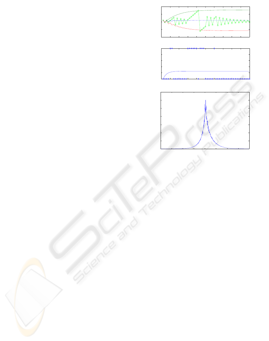
0 5 10 15 20 25 30 35 40 45 50

−10

−5

Continuous−Valued State: Sample Run and Statistics

Time

Sample Run, Mean,

and 2 σ Bounds

0 5 10 15 20 25 30 35 40 45 50

0.2

0.4

0.6

0.8

Underlying Markov Chain Status

Time

Sample Run and

Prob. of Status "1"

−20 −15 −10 −5 0 5 10 15 20

0.002

0.004

0.006

0.008

0.01

0.012

0.014

Steady−State Distribution

Continuous−Valued State

Probability Distribution

Mean = 0.92

St. Dev.=3.4

Skewness=3.8

Figure 1: This ﬁgure illustrates the MLSS-based analy-

sis of moments for an example MJLS. The top plot in

this ﬁgure speciﬁes the continuous-valued state during a 50

time-step simulation, along with the computed mean value

and two standard deviation intervals for this continuous-

valued state. The middle plot indicates the status of the

underlying Markov chain during the simulation and also

shows the probability that the Markov chain is in status “1”.

The bottom plot shows the steady-state distribution for the

continuous-valued state (found through iteration of the dis-

tribution) and lists the moments of this continuous-valued

state (found with much less computation using the moment

recursions).

example MJLS, with statistics shown in Fig. 1, can

be shown to be moment-convergent. Our study of

moment convergence complements stability studies

for MJLS (e.g., (Fang and Loparo, 2002)), by allow-

ing identiﬁcation of MJLS whose moments reach a

steady-state but that are not stable (in the sense that

state itself does not reach a steady-state).

The MLSS reformulation can be used to develop

LMMSE estimators for MJLS. LMMSE estimation of

the continuous-valued state of an MJLS from noisy

observations has been considered by (Costa, 1994).

The observation structure (i.e., the generator of the

observation from the concurrent state) assumed by

(Costa, 1994) can be captured using our MLSS for-

mulation, and in that case our estimator is nearly iden-

tical to that of (Costa, 1994); only the squared error

that is minimized by the two estimators is slightly dif-

ferent.

MOMENT-LINEAR STOCHASTIC SYSTEMS

195

Our MLSS formulation allows for estimation for a

variety of observation structures. For instance, we can

capture observations that are Poisson random vari-

ables, with parameter equal to a linear function of

the state variables. (Such an observation model may

be realistic, for example, if the state process modu-

lates an observed Poisson arrival process.) We can

also capture other types of state-dependent noise in

the observation process, as well as various discrete

and continuous-valued state-independent noise. Fur-

ther, hybrids of multiple observation structures can be

captured in the MLSS formulation.

Another potential advantage of the MLSS formula-

tion is that, because the underlying Markov status is

part of the state vector, this underlying status can be

estimated. The accuracy of our estimator for the un-

derlying state remains to be assessed. A direction for

future study is to compare our estimator for the un-

derlying status with the nonlinear estimators of, e.g.,

(Sworder et al., 2000; Mazor et al., 1998).

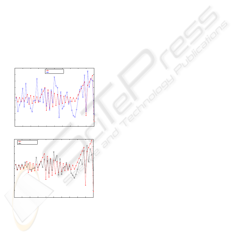
0 5 10 15 20 25 30 35 40 45 50

−8

−6

−4

−2

Time

x[k] and y[k]

Continuous State and Observations

State x[k]

Observation y[k]

0 5 10 15 20 25 30 35 40 45 50

−8

−6

−4

−2

Time

x[k] and \hat{x}[k]

Continuous State and Estimate

State x[k]

Estimate \hat{x}[k]

Figure 2: In the left plot, the continuous-valued state and

observations during a 50 time-step simulation of the exam-

ple MJLS are shown. In the right plot, the LMMSE estimate

for the continuous-valued state is compared with the actual

continuous-valued state. The LMMSE estimate is a better

approximation for the continuous-valued state than the ob-

servation sequence.

For illustration, we have developed an LMMSE

ﬁlter for our example MJLS. Here, we observe the

(scalar) continuous-valued state upon corruption by

additive white Gaussian noise. Fig. 2 illustrates the

performance of the LMMSE estimator, for a partic-

ular sample run. Our analysis shows that the error

covariance of our estimate is about half the measure-

ment error covariance, verifying that our estimate is

usually a more accurate estimate for the state than the

unﬁltered observation sequence.

5 MLSS MODELS FOR

NETWORK DYNAMICS:

SUMMARY

We believe that MLSS representations for networks

are of special interest because analysis of stochastic

network dynamics is quite often computationally in-

tensive (e.g., exponential in the number of vertices),

while MLSS representations can permit analysis at

much lower computational cost. Below, we summa-

rize our studies of MLSS representations for network

dynamics. More detailed description of MLSS mod-

els for network dynamics can be found in (Roy, 2003).

The following are examples of MLSS models for

network dynamics that we have considered.

• The inﬂuence model was introduced in (Asavathi-

ratham, 2000) as a network of interacting ﬁnite-

state Markov chains, and is developed and mo-

tivated in some detail in (Asavathiratham et al.,

2001). We refer the reader to (Basu et al., 2001)

for one practical application, as a model for con-

versation in a group. The inﬂuence model consists

of sites with discrete-valued statuses that evolve in

time through stochastic interaction. The inﬂuence

model’s structured stochastic update permits for-

mulation of the model as an MLSS, using 0–1 in-

dicator vector representations for each site’s status.

The rth moment recursion permits computation of

the joint probabilities of the statuses of groups of r

sites, and hence the conﬁgurations of small groups

of sites can be characterized using low-order re-

cursions. The MLSS formulation for the inﬂuence

model can also be used to develop good state esti-

mators for the model, and to prove certain results

on the convergence of the model.

• MLSS can be used to represent single-server

queueing networks with linear queue length-

dependent arrival and service rates, operating under

heavy-trafﬁc conditions. The MLSS formulation

allows us to ﬁnd statistics and cross-statistics of the

queue lengths. Of particular interest is the possi-

bility for using the MLSS formulation to develop

queue-length estimators for these state-dependent

models and, indirectly, for Jackson networks (see,

e.g., (Kelly, 1979)).

ICINCO 2004 - SIGNAL PROCESSING, SYSTEMS MODELING AND CONTROL

196

• In (Roy et al., 2004), we have developed an MLSS

model for aircraft counts in regions of the U.S.

airspace, and have used the MLSS formulation to

compute statistics of aircraft counts in regions. In

the context of this MLSS model, we have also de-

veloped techniques for parameter estimation from

data.

REFERENCES

Asavathiratham, C. (2000). The Inﬂuence Model: A

Tractable Representation for the Dynamics of Net-

worked Markov Chains, Ph.D. Thesis. EECS Depart-

ment, Massachusetts Institute of Technology.

Asavathiratham, C., Roy, S., Lesieutre, B. C., and Verghese,

G. C. (2001). The inﬂuence model. IEEE Control

Systems Magazine.

Baiocchi, A., Melazzi, N. B., Listani, M., Roveri, A., and

Winkler, R. (1991). Loss performance analysis of

an ATM multiplexer loaded with high-speed on off

sources. IEEE Journal on Selected Areas of Commu-

nications, 9:388–393.

Basu, S., Choudhury, T., Clarkson, B., and Pentland, A.

(2001). Learning human interactions with the inﬂu-

ence model. MIT Media Lab Vision and Modeling

TR#539.

Bose, A. (2003). Power system stability: new opportuni-

ties for control. Stability and Control of Dynamical

Systems with Applications.

Catlin, D. E. (1989). Estimation, Control, and the Discrete

Kalman Filter. Springer-Verlag, New York.

Ching, W. K. (1997). Markov-modulated Poisson processes

for multi-location inventory problems. International

Journal of Production Economics, 52:217–233.

Chizeck, N. J. and Ji, Y. (1988). Optimal quadratic con-

trol of jump linear systems with Gaussian noise in

discrete-time. Proceedings of the 27th IEEE Confer-

ence on Decision and Control, pages 1989–1999.

Costa, O. L. V. (1994). Linear minimum mean square er-

ror estimation for discrete-time markovian jump lin-

ear systems. IEEE Transactions on Automatic Con-

trol, 39:1685–1689.

Durrett, R. (1981). An introduction to inﬁnite particle sys-

tems. Stochastic Processes and their Applications,

11:109–150.

Fang, Y. and Loparo, K. A. (2002). Stabilization of

continuous-time jump linear systems. IEEE Transac-

tions on Automatic Control, 47:1590–1603.

Fang, Y., Loparo, K. A., and Feng, X. (1991). Modeling is-

sues for the control systems with communication de-

lays. Ford Motor Co., SCP Research Report.

Heskes, T. and Zoeter, O. (2003). Generalized belief propa-

gation for approximate inference in hybrid bayesian

networks. Proceedings of the Ninth International

Workshop on Artiﬁcial Intelligence and Statistics.

Kelly, F. P. (1979). Reversibility and Stochastic Networks.

John Wiley and Sons, New York.

Loparo, K. A., Buchner, M. R., and Vasuveda, K. (1991).

Leak detection in an experimental heat exchanger pro-

cess: a multiple model approach. IEEE Transations on

Automatic Control, 36.

Mazor, E., Averbuch, A., Bar-Shalom, Y., and Dayan, J.

(1998). Interacting multiple model methods in target

tracking: a survey. IEEE Transactions on aerospace

and electronic systems, 34(1):103–123.

Mendel, J. M. (1975). Tutorial on higher-order statistics

(spectra) in signal processing and system theory: the-

oretical results and some applications. Proceedings of

the IEEE, 3:278–305.

Meyn, S. and Tweedie, R. (1994). Markov

Chains and Stochastic Stability.

http://black.csl.uiuc.edu/ meyn/pages/TOC.html.

Nagarajan, R., Kurose, J. F., and Towsley, D. (1991). Ap-

proximation techniques for computing packet loss in

ﬁnite-buffered voice multiplexers. IEEE Journal on

Selected Areas of Communications, 9:368–377.

Rabiner, L. R. (1986). A tutorial on hidden markov models

and selected applications in speech recognition. Pro-

ceedings of the IEEE, 77(2):257–285.

Rothman, D. and Zaleski, S. (1997). Lattice-Gas Cellular

Automata: Simple Models of Complex Hydrodynam-

ics. Cambridge University Press, New York.

Roy, S. (2003). Moment-Linear Stochastic Systems and

their Applications. EECS Department, Massachusetts

Institute of Technology.

Roy, S., Verghese, G. C., and Lesieutre, B. C. (2004).

Moment-linear stochastic systems and networks. Sub-

mitted to the Hybrid Systems Computation and Con-

trol conference.

Segall, A., Davis, M. H., and Kailath, T. (1975). Nonlinear

ﬁltering with counting observations. IEEE Transac-

tions on Information Theory, IT-21(2).

Snyder, D. L. (1972). Filtering and detection of doubly

stochastic poisson processes. IEEE Transactions on

Information Theory, IT-18:91–102.

Swami, A. and Mendel, J. M. (1990). Time and lag re-

cursive computation of cumulants from a state space

model. IEEE Transactions on Automatic Control,

35:4–17.

Sworder, D. D., Boyd, J. E., and Elliot, R. J. (2000). Modal

estimation in hybrid systems. Journal of Mathemati-

cal Analysis and Applications, 245:225–247.

Zehnwirth, B. (1988). A generalization of the Kalman ﬁl-

ter for models with state-dependent observation vari-

ance. Journal of the American Statistical Association,

83(401):164–167.

MOMENT-LINEAR STOCHASTIC SYSTEMS

197

REFERENCES

Asavathiratham, C. (2000). The Influence Model: A