REALISTIC DYNAMIC SIMULATION OF AN INDUSTRIAL ROBOT

WITH JOINT FRICTION

Ronald G.K.M. Aarts, Ben J.B. Jonker

University of Twente, Faculty of Engineering Technology

Enschede, The Netherlands

Rob R. Waiboer

Netherlands Institute for Metals Research

Delft, The Netherlands

Keywords:

Realistic closed-loop trajectory simulation, Industrial robot, Perturbation method, Friction modelling.

Abstract:

This paper presents a realistic dynamic simulation of the closed-loop tip motion of a rigid-link manipulator

with joint friction. The results from two simulation techniques are compared with experimental results. A

six-axis industrial St

aubli robot is modelled. The LuGre friction model is used to account both for the sliding

and pre-sliding regime. The manipulation task implies transferring a laser spot along a straight line with a

trapezoidal velocity proﬁle.

Firstly, a non-linear ﬁnite element method is used to formulate the dynamic equations of the manipulator

mechanism. In a closed-loop simulation the driving torques are generated by the control system. The computed

trajectory tracking errors agree well with the experimental results. Unfortunately, the simulation is very time-

consuming due to the small time step of the discrete-time controller.

Secondly, a perturbation method has been applied. In this method the perturbed motion of the manipulator is

modelled as a ﬁrst-order perturbation of the nominal manipulator motion. Friction torques at the actuator joints

are introduced at the stage of perturbed dynamics. A substantial reduction of the computer time is achieved

without loss of accuracy.

1 INTRODUCTION

Robotic manipulators for laser welding must pro-

vide accurate path tracking performance of 0.1 mm

and less at relatively high tracking speed exceed-

ing 100 mm/s. High speed manipulator motions are

accompanied by high-frequency vibrations of small

magnitudes whereas velocity reversals in the joints

lead to complicated joint friction effects. These dy-

namic phenomena may signiﬁcantly effect the weld

quality, since laser welding is sensitive to small varia-

tions in the processing conditions like welding speed

as well as to disturbances of the position of the laser

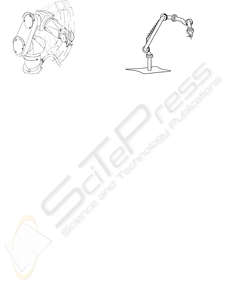
spot with respect to the seam to be welded. To study

the applicability of industrial robotic manipulators as

in Fig. 1 for laser welding tasks, a framework for real-

istic dynamic simulations of the robot motion is being

developed. Such a simulation should predict the path

tracking accuracies, thereby taking into account the

dynamic limitations of the robotic manipulator such

as joint ﬂexibility, friction and limits of the drive sys-

tem like the maximum actuator torques. Obviously

the accuracy of the simulation has to be sufﬁciently

high with respect to the allowable path deviations.

Unfortunately, closed-loop dynamic simulations

with a sufﬁcient degree of accuracy are computation-

ally expensive and time consuming especially when

static friction, high-frequency elastic modes and a

digital controller operating with small discrete time

steps are involved. In an earlier paper we discussed

a so-called perturbation method (Jonker and Aarts,

2001) which proved to be accurate and computation-

ally efﬁcient for simulations of robotic manipulators

with ﬂexible links. In this paper a similar perturbation

scheme is presented for the closed-loop dynamic sim-

ulation of a rigid-link manipulator with joint friction.

The extension to an industrial robot with elastic joints

is still a topic of ongoing research.

We consider the motion of a six axes industrial

robot (St

aubli RX90B), Fig. 1. The unknown robot

manipulator parameters, such as inertias of the ma-

nipulator arms, the stiffness and the pretension of a

gravity compensation spring are determined by means

of parameter identiﬁcation techniques. The friction

characteristics are identiﬁed separately. The con-

troller model is based on manufacturer’s data and has

been veriﬁed experimentally using system identiﬁca-

tion techniques. Details of the identiﬁcation tech-

Aarts R., Jonker B. and Waiboer R. (2004).

REALISTIC DYNAMIC SIMULATION OF AN INDUSTRIAL ROBOT WITH JOINT FRICTION.

In Proceedings of the First Inter national Conference on Informatics in Control, Automation and Robotics, pages 48-55

DOI: 10.5220/0001143500480055

 SciTePress

Axis 1

Axis 2

Axis 3

Axis 4

Axis 5

Axis 6

Figure 1: The six axes St

aubli RX90B Industrial robot

Axis 5

Hinge 1 (q

)

Hinge 2 (q

)

Hinge 3 (q

)

Hinge 4 (q

)

Hinge 5 (q

)

Hinge 6 (q

)

End-effector

Base

Beam 1

Beam 2

Beam 3

Beam 4

Beam 5

Beam 6

Truss 1 (k

, σ

(c,0)

)

Figure 2: The 6 DOF Finite Element Model.

niques are outside the scope of this paper and will be

outlined elsewhere (Waiboer, 2004).

The present paper will focus on two simulation

techniques and a comparison of numerical and exper-

imental results. At ﬁrst, a non-linear ﬁnite element

method (Jonker, 1990) is used to formulate the dy-

namic equations of the manipulator mechanism, sec-

tion 2. The ﬁnite element formulation and the pro-

posed solution method are implemented in the pro-

gram SPACAR (Jonker and Meijaard, 1990). An inter-

face to MAT LAB is available and the closed-loop sim-

ulations are carried out using SIMULIN K’s graphical

user interface. A driving system is added to the ma-

nipulator model, section 3, and the inﬂuence of joint

friction is taken into account, section 4. The LuGre

friction model (Wit et al., 1995) has been used as it

accounts for both the sliding and pre-sliding regimes.

Finally the closed-loop model is assembled by includ-

ing the control system, section 5.

The second approach is the so-called perturbation

method, section 6. The differences between the actual

manipulator motion and the nominal (desired) motion

are modelled as ﬁrst order perturbations of that nomi-

nal motion. The computation of the perturbed motion

is carried out in two steps. In the ﬁrst step, the ﬁnite

element method permits the generation of locally lin-

earised models (Jonker and Aarts, 2001). In the sec-

ond step, the linearised model can simulate the per-

turbed motion of the manipulator accurately as long

as it remains sufﬁciently close to the nominal path.

The perturbation method is computationally more ef-

ﬁcient as the non-linear model only has to solved dur-

ing the ﬁrst step in a limited number of points along

the nominal trajectory. This is the solution of an in-

verse dynamic analysis along a known path, so with

only algebraic equations. The friction torques at the

actuator joints and the control system are introduced

at the stage of perturbed dynamics in the second step.

In section 7, the simulation results will be compared

with the experimental results. Also results acquired

with the perturbation method will be compared with

those obtained from a full non-linear dynamic simu-

lation.

2 FINITE ELEMENT

REPRESENTATION OF THE

MANIPULATOR

In the non-linear ﬁnite element method, a manipu-

lator mechanism is modelled as an assembly of ﬁ-

nite elements interconnected by joint elements such

as hinge elements and (slider) truss elements. This

is illustrated in Fig. 2, where the St

aubli robot with

six degrees of freedom is modelled by three different

types of elements. The gravity compensation spring

is modelled as a slider-truss element. The manipu-

lator arms are modelled by beam elements. Finally,

the joints are represented by six cylindrical hinge ele-

ments, which are actuated by torque servos. The ma-

nipulator mechanism is assembled by allowing the el-

ements to have nodal points in common. The con-

ﬁguration of the manipulator is then described by the

vector of nodal coordinates x, some of which may

be the Cartesian coordinates, while others describe

the orientation of orthogonal triads rigidly attached

at the element nodes. The motion of the manipulator

mechanism is described by relative degrees of free-

dom which are the actuator joint angles denoted by

the vector q. By means of the geometric transfer func-

tions F

(x)

and F

(e,c)

, the nodal coordinates x and the

elongation of the gravity compensating spring e

(c)

are

expressed as functions of the joint angles q

x = F

(x)

(q) (1)

and

(c)

= F

(e,c)

(q) . (2)

REALISTIC DYNAMIC SIMULATION OF AN INDUSTRIAL ROBOT WITH JOINT FRICTION

Differentiating the transfer functions with respect to

time gives

x = DF

(x)

q (3)

and

˙e

(c)

= DF

(e,c)

q, (4)

where the differentiation operator D represents partial

differentiation with respect to the degrees of freedom.

The acceleration vector

x is obtained by differentiat-

ing (3) again with respect to time,

x = DF

(x)

q + (D

(x)

q. (5)

The geometric transfer functions F

(x)

and F

(e,c)

are

determined numerically in an iterative way (Jonker,

1990).

The inertia properties of the concentrated and dis-

tributed mass of the elements are described with the

aid of lumped mass matrices. Let M(x) be the global

mass matrix, obtained by assembling the mass matri-

ces of the individual elements and let f (x,

x, t) be

the global force vector including gravity forces and

the velocity dependent inertia forces. Then the equa-

tions of motion described in the dynamic degrees of

freedom are given by

q + DF

(x)T

M(D

(x)

q − f

+ DF

(e,c)T

(c)

= τ ,

(6)

where

M = DF

(x)T

MDF

(x)

is the reduced mass

matrix and σ

(c)

is the total stress in the gravity com-

pensating spring. The vector τ represents the joint

driving torques. The constitutive relation for the grav-

ity compensating spring is described by

(c)

= σ

(c,0)

+ k

(c)

, (7)

where σ

c,0

and k

denote the pre-stress and the stiff-

ness coefﬁcients of the spring, respectively.

This ﬁnite element method has been implemented

in the SPACAR software program (Jonker and Mei-

jaard, 1990).

3 THE DRIVING SYSTEM

The robot is driven by servo motors connected via

gear boxes to the robot joints. The inputs for the drive

system are the servo currents i

and the outputs are the

joint torques τ

, where the subscript j = 1..6 denotes

either the motor or the joint number. A schematic

model of the drives of joints 1 to 4 is shown in Fig. 3.

The relations between the vector of motor angles ϕ,

the vector of joint angles q and their time derivatives

are given by

ϕ = Tq, (8)

ϕ = T

q, (9)

ϕ = T

q, (10)

(m)

(f )

Figure 3: Schematic representation of the drives for joints 1

to 4.

where T is the transmission model for the joints. For

joints j = 1..5 only the respective gear ratio n

of the

joint plays a role. The drives for the wrist of the robot,

drives 5 and 6, are coupled. This causes an extra term

leading to

T =







0 0 0 0 0

0 n

0 0 0 0

0 0 n

0 0 0

0 0 0 n

0 0

0 0 0 0 n







. (11)

The friction torque in each joint is denoted τ

(f)

with

j = 1..6. Due to the coupling in the wrist, an addi-

tional friction torque τ

(f)

is identiﬁed on the axis of

motor 6. The vector of joint friction torques is then

deﬁned as

(f)

, τ

(f)

, τ

(f)

, τ

(f)

, · · ·

(f)

+τ

(f)

, τ

(f)

+τ

(f)

(12)

The joint friction modelling is continued in section 4.

The drives are equipped with permanent magnet,

three-phase synchronous motors, yielding a linear re-

lation between motor currents and torque. The vector

of joint driving torques τ is then given by

τ = T

(m)

i − T

(m)

ϕ − τ

(f)

, (13)

where the matrices C

(m)

and J

(m)

are diagonal ma-

trices with the motor constants c

(m)

and rotor inertias

(m)

, respectively. Substitution of (10) and (13) into

(6) and some rearranging yields

(n)

q + DF

(x)T

M(D

(x)

q − f

+ DF

(e,c)T

(c)

= τ

(n)

(14)

where the mass matrix

(n)

is deﬁned by

(n)

M + T

(m)

T , (15)

as the rotor inertias T

(m)

T obviously have to be

added to the reduced mass matrix

M in the equations

of motion (6). Furthermore, the vector of net joint

torques is deﬁned as

(n)

= T

(m)

i − τ

(f)

. (16)

The inertia properties and spring coefﬁcients have

been found by means of parameter identiﬁcation tech-

niques (Waiboer, 2004).

ICINCO 2004 - ROBOTICS AND AUTOMATION

4 JOINT FRICTION MODEL

For feed-forward dynamic compensation purposes

and robot inertia identiﬁcation techniques it is com-

mon to model friction in robot joints as a torque τ

(f)

which consists of a Coulomb friction torque and an

additional viscous friction torque for non-zero veloc-

ities (Swevers et al., 1996; Calaﬁore et al., 2001).

These so-called static or kinematic friction models

are valid only at sufﬁciently high velocities because

they ignore the presliding regime. At zero velocity

they show a discontinuity in the friction torque which

gives rise to numerical integration problems in a for-

ward dynamic simulation. To avoid this problem we

apply the LuGre friction model (Wit et al., 1995), that

accounts for both the friction in the sliding and in the

presliding regime.

In the LuGre friction model there is an internal state

z that describes the average presliding displacement,

as introduced by Heassig et al. (Haessig and Fried-

land, 1991). The state equations with a differential

equation for the state z and an output equation for the

friction moment τ

(f)

are

˙z = ˙q −

| ˙q |

g( ˙q)

z, (17)

(f)

= c

(0)

z + c

(1)

˙z + c

(2)

˙q . (18)

Note that a subscript j = 1 . . . 7 should be added to all

variables to distinguish between the separate friction

torques in the robot model, but it is omitted here for

better readability. For each joint friction model with

j = 1..6 the input velocity equals the joint velocity ˙q

For the extra friction model τ

(f)

the input velocity is

deﬁned as the sum of the joint velocities of joints 5

and 6.

In general, the friction torque in the pre-sliding

regime is described by a non-linear spring-damper

system that is modelled with an equivalent stiffness

(0)

for the position–torque relationship at velocity re-

versal and a micro-viscous damping coefﬁcient c

(1)

At zero velocity, the deformation of the non-linear

spring torque is related to the joint (micro) rotation

The viscous friction torque in the sliding regime is

modelled by c

(2)

˙q, where c

(2)

is the viscous friction

coefﬁcient. In addition, at a non-zero constant veloc-

ity ˙q, the internal state z, so the average deformation,

will approach a steady state value equal to c

(0)

g( ˙q).

The function g( ˙q) can be any function that represents

the constant velocity behaviour in the sliding regime.

In this paper the Stribeck model will be used, which

models the development of a lubricating ﬁlm between

the contact surfaces as the relative velocity increases

from zero. The Stribeck model is given by

(0)

g( ˙q) = τ

(c)

+ (τ

(s)

− τ

(c)

−(| ˙q|/ω

)

, (19)

where τ

(c)

is known as Coulomb friction torque, τ

(s)

is the static friction torque and ω

and δ are shaping

parameters. The values for the static friction torque

(s)

and Coulomb friction torque τ

(c)

may be differ-

ent for positive and negative velocities and are there-

fore distinguished by the subscripts + and −, respec-

tively.

For each friction torque in the robot model, the

parameters describing the sliding regime of the Lu-

Gre friction model are estimated separately using

dedicated joint torque measurements combined with

non-linear parameter optimisation techniques (Wai-

boer, 2004). The parameters describing the pre-

sliding regime are approximated by comparing the

pre-sliding behaviour in simulation with measure-

ments.

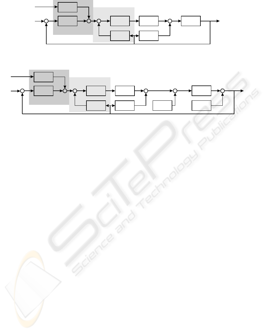
5 CLOSED-LOOP ROBOT

MODEL

The SPAC A R model of the manipulator mechanism,

the controller, the friction models and the robot drives

are assembled into a complete model of the closed-

loop robot system, Fig. 4.

The CS7B controller used in the St

aubli RX90B

is an industrial PID controller based on the Adept

V+ operating- and motion control system. The con-

troller includes six SISO controllers, one for each

servo-motor. A trajectory generator computes the set-

points ¨q

(r)

, ˙q

(r)

and q

(r)

at a rate of 1 kHz. The

actual joint position q is compared with the set-point

(r)

and the error ² is fed into the P I-block of the

controller, which includes the proportional part and

the integrator part. The acceleration set-points

(r)

and velocity set-points

(r)

are used for accelera-

tion feed-forward and friction compensation, both in-

cluded in the F F -block. The friction compensation

includes both Coulomb and viscous friction. The ve-

locity feedback

q is fed into the D-block, represent-

ing the differential part of the control scheme. The

block C represents the current loop, including the

power ampliﬁer. Note that the position loop runs

at f

(1)

= 1 kHz and the velocity loop and current

loop run at f

(2)

= 4 kHz. The transfer functions

of the different blocks have been identiﬁed and im-

plemented in a SI MULINK block scheme of the robot

controller (Waiboer, 2004).

The current vector i is fed into the drive model

where the joint torques are computed. The LuGre

friction models compute the friction torques from

the joint velocities

q. The net joint torque τ

(n)

(14) is the input for the non-linear manipulator model

(SPACAR). The output of the manipulator model con-

tains the joint positions, and velocities, denoted by q

REALISTIC DYNAMIC SIMULATION OF AN INDUSTRIAL ROBOT WITH JOINT FRICTION

−

(r)



(n)

(f)

(1)

= 1kHz

(2)

= 4kHz

F F

P I

Drives

Friction

SPACAR

Figure 4: Assembly of the closed-loop robot model for a simulation with the non-linear ﬁnite element method (SPACAR

block).

−

(r)



F F

P I

Drives

Friction

(n)

(f)

= 1kHz

= 4kHz

read y

δy

δτ

(n)

read τ

LT V

Figure 5: Perturbation scheme with the linearised equations of motion (LTV block).

and

q, respectively.

6 PERTURBATION METHOD

In the presented closed-loop model, both the SPACAR

model and the friction model are continuous in time,

while the controller sections are discrete and running

at 1 kHz and 4 kHz, respectively. In SIMULINK this

implies that the SPACAR model is simulated at a time

step equal to 0.25 ms or even smaller if this is re-

quired by SIMUL I NK’s integrator. Due to the fact that

the position, computed within the SPACAR simulation

model, is obtained in an iterative way, the computa-

tion effort is quite elaborate. This results in long sim-

ulation times. In order to overcome this drawback,

the perturbation method (Jonker and Aarts, 2001) is

applied.

In the perturbation method, deviations from the

(nominal) desired motion (q

) due to joint

friction and errors of the control system are modelled

as ﬁrst-order perturbations (δq, δ

q, δ

q) of the nomi-

nal motion, such that the actual variables are of the

form:

q = q

+ δq, (20)

q =

+ δ

q, (21)

q =

+ δ

q, (22)

where the preﬁx δ denotes a perturbation. Expanding

(1) and (3) in their Taylor series expansion and disre-

garding second and higher order terms results in the

linear approximations

δx = DF

·δq, (23)

x = DF

·δ

q + (D

)·δq. (24)

The subscript 0 refers to the nominal trajectory.

The nominal motion is computed ﬁrst and is de-

scribed by the non-linear manipulator model. The

non-linear equations of motion (14) for the nominal

motion become

(n)

+ D

·(

))·(

) − f

+ DF

(e,c)

(c)

= τ

(n)

(25)

where σ

(c)

= σ

(c,0)

+ k

(c)

. The right hand side

vector τ

(n)

represents the nominal net input torque

necessary to move the manipulator along the nomi-

nal (desired) trajectory. It is determined from an in-

verse dynamic analysis based on (25). Note that τ

(n)

is computed without the presence of friction. Obvi-

ously, the desired nominal motion (

, q

) equals

the reference motion (

(r)

, q

(r)

) of the closed

loop system.

Next the perturbed motion is described by a set

of linear time-varying equations of motion, which

are obtained by linearising the equations of motion

around a number of points on the nominal trajectory.

The resulting equations of motion for the perturba-

tions of the degrees of freedom δq are

(n)

q + C

q +

δq = δτ

(n)

, (26)

where

(n)

is the reduced system mass matrix as in

(14), C

is the velocity sensitivity matrix. Matrix

is a shorthand notation for the combined stiffness ma-

trices

= K

+ N

+ G

, (27)

ICINCO 2004 - ROBOTICS AND AUTOMATION

where K

denotes the structural stiffness matrix, N

and G

are the dynamic stiffening matrix and the ge-

ometric stiffening matrix, respectively. The matrices

(n)

, K

and G

are symmetric, but C

and N

need not to be symmetrical. Expressions for these

matrices are given in (Jonker and Aarts, 2001).

Fig. 5 shows the block scheme of the closed-loop

perturbation model. Note that the non-linear manip-

ulator model (SPACAR) is replaced by the LTV-block

which solves (26). Its input δτ

(n)

is computed ac-

cording to

δτ

(n)

= τ

(n)

− τ

(n)

, (28)

where τ

(n)

represents the vector of the net joint

torques as deﬁned by (16). The perturbed output vec-

tor δy is added to the output vector y

of the nominal

model, yielding the actual output y. This output vec-

tor will be discussed below.

Within the SIMULINK framework the LTV block

represents a linear time-varying state space represen-

tation of a system

= A

+ B

= C

(29)

where u

, y

and x

are the input, output and state

vectors, respectively, and A

, B

and C

are the

time-varying state space matrices. Equation (26) is

written in this representation by deﬁning the state and

input vectors

= [δ

q, δq]

= δτ

(n)

(30)

The state space matrices A

and B

are then com-

puted from the matrices in (26) using a straightfor-

ward procedure :

0 I

−

(n)

−1

−

(n)

−1

(n)

−1

(31)

The output matrix C

depends on the output vector

that is deﬁned by the user. It may consist of (ﬁrst

derivatives of) the degrees of freedom δq present in

or (ﬁrst derivatives of) nodal coordinates δx that

are computed from x

using (23) and (24). E.g. the

coordinates δx in y

are computed using

= [

] . (32)

For a practical implementation of the perturba-

tion method the total trajectory time T is divided

into intervals. The state space matrices and the vec-

tors τ

and y

are computed during a preprocess-

ing run at a number N of discrete time steps t = t

(i = 0, 1, 2, ..., N ) and stored in a ﬁle. During the

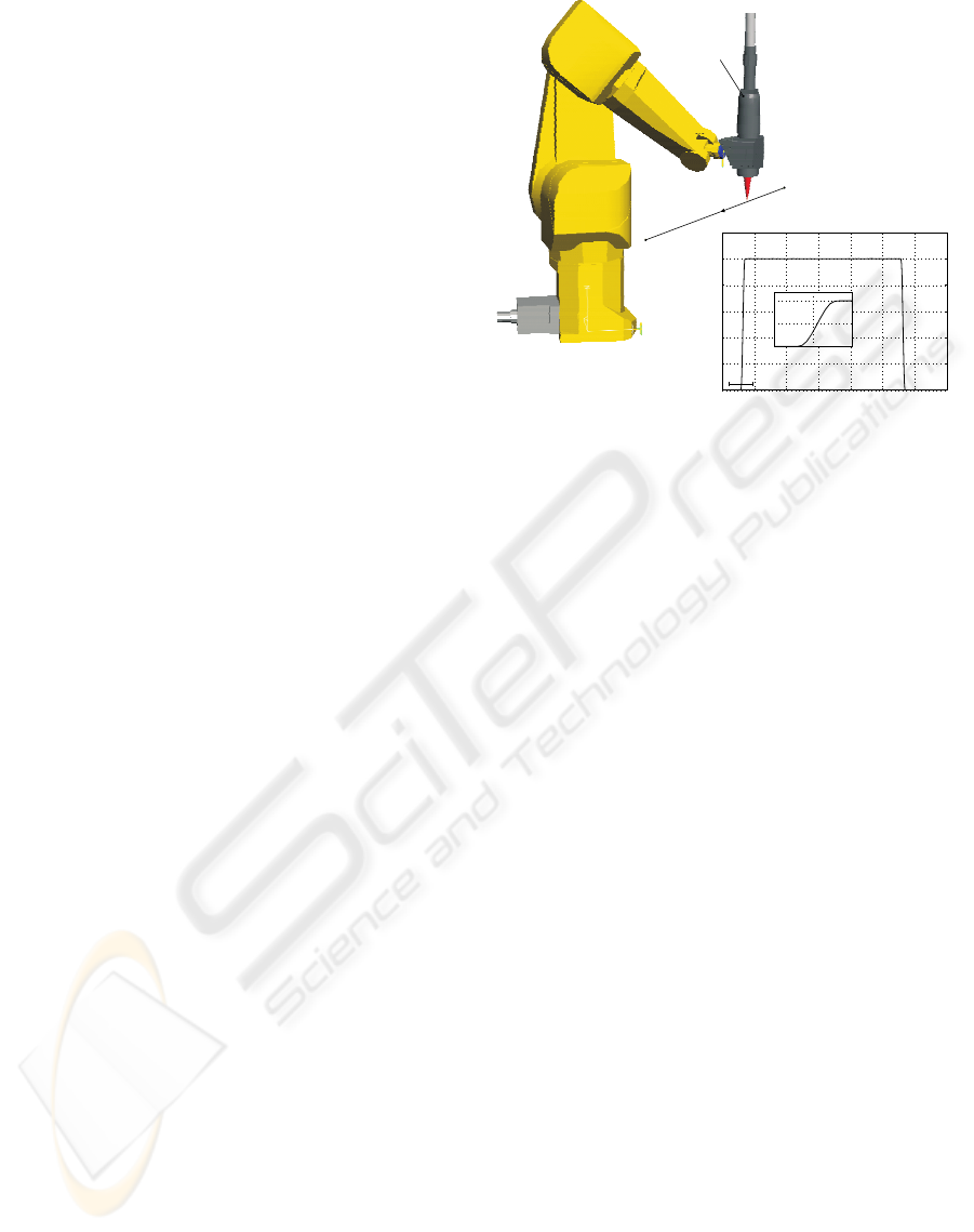
Welding

head

2 4

6 8 10

12 14

1.25 1.5

100

120

time [s]

Tip velocity [mm/s]





Figure 6: The simulated straight line path and the path ve-

locity.

simulation runs the matrices and vectors are then read

back from this ﬁle. Between two time steps the co-

efﬁcients of the state space matrices are interpolated

linearly. Cubic interpolation is used for the vectors τ

and y

7 SIMULATION RESULTS

In Fig. 6 an experiment is deﬁned in which a straight

line motion of the robot tip has to be performed in the

horizontal plane with a velocity proﬁle as presented

in the insert. The welding head remains in the verti-

cal position as shown in Fig. 6. The joint set-points

are computed with the inverse kinematics module of

the SPACAR software. The joint velocities are shown

in Fig. 7. The ﬁgures show clearly the non-linear be-

haviour of the robot. Note the velocity reversal of

joints 2 and 3 nearly halfway the trajectory.

First, the trajectory will be simulated with the non-

linear model. The simulation has been performed in

SIMULIN K using the ode23tb integration scheme,

which is one of the stiff integrators in SIMULIN K.

The stiff integration scheme is needed due to the high

equivalent stiffness in the pre-sliding part of the fric-

tion model (18).

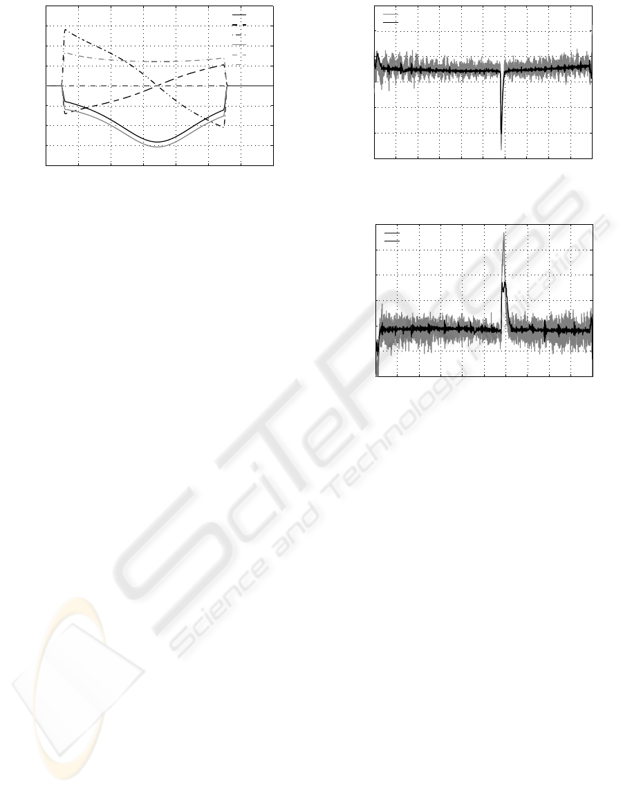
The path performance as predicted by the model

will be compared to measurements carried out on the

actual robot. In both the measurements and simula-

tions, the path position is based on joint axis positions

and the nominal kinematic model. In Fig. 8, the hor-

izontal and vertical path deviations are shown. The

results show that the agreement between the simu-

lated prediction and the measurement is within 20 µm

REALISTIC DYNAMIC SIMULATION OF AN INDUSTRIAL ROBOT WITH JOINT FRICTION

6 8 10

−0.4

−0.3

−0.2

−0.1

0.1

0.2

0.3

0.4

time [s]

V elocity [rad/s]

Figure 7: The joint velocity.

which is well within the range of accuracy required

for laser welding. At about 600 mm on the trajec-

tory, at the velocity reversal in joints 2 and 3, there is

a jump of the friction force, resulting in a relatively

large path error.

During the experiment the motor currents were

recorded. In Fig. 9 the measured motor currents of

joint 3 is compared with the simulated motor current

as an example. The simulation shows good agreement

with the measurements. It can be observed that the

motor currents are predicted quite accurately in the

sliding regime and near the velocity reversal. How-

ever, the model is unable to predict the stick-torques

with a high level of accuracy. This can be explained

by the fact that the stiction torque can be anywhere be-

tween τ

(s)

−

and τ

(s)

over a very small position range

of tenths of µrad, due to the high equivalent stiffness

(0)

in (18).

The required simulation time with the non-linear

simulation model was about 70 minutes on a 2.4 GHz

Pentium 4 PC, which indicates that it is computation-

ally quite intensive. This is caused by the small time

steps at which the manipulator conﬁguration, see (1)

and (2), needs to be solved by an iterative method. To

overcome this drawback, the perturbation approach

will be used next.

For the perturbation method the number of points

along the trajectory N at which the system is lin-

earised is taken to be 400. The simulation results of

the perturbation method and the non-linear simulation

have been compared. Fig 10 shows the path accuracy

along the trajectory. There is no noticeable difference

between the results at this scale. The error stays well

below 10 µm and is mostly less than 2 µm. Also the

agreement between the simulated motor currents for

both the non-linear simulation and the perturbation

method is good, especially when the manipulator is in

motion. At rest, the torques in the stick or pre-sliding

regime shows some differences as before. A signiﬁ-

cant reduction of simulation time by about a factor 10

0 200 400 600 800 1000

−0.08

−0.06

−0.04

−0.02

0.02

0.04

Measurement

Simulation

position [mm]

deviation [mm]

a. Horizontal deviation.

a. Horizontal deviation

0 200 400 600 800 1000

0.08

0.06

0.04

0.02

−0.02

−0.04

Measurement

Simulation

position [mm]

deviation [mm]

b. Vertical deviation.

b. Vertical deviation

Figure 8: Simulated and measured path deviation.

has been achieved.

8 CONCLUSIONS

In this paper a realistic dynamic simulation of a rigid

industrial robot has been presented. The following

components are essential for the closed-loop simula-

tion:

• A ﬁnite element-based robot model has been used

to model the mechanical part of the robot. Robot

identiﬁcation has been applied to ﬁnd the model pa-

rameters accurately.

• Furthermore, joint friction has been modelled using

the LuGre friction model.

• Finally, a controller model has been identiﬁed and

implemented.

The complete closed-loop model has been used for

the simulation of the motion of the robot tip along

a prescribed trajectory. The simulation results show

good agreement with the measurements. It was

found that a closed-loop simulation with the non-

linear robot model was very time consuming due

ICINCO 2004 - ROBOTICS AND AUTOMATION

6 8 10

−900

−800

−700

−600

−500

−400

−300

−200

−100

100

time [s]

Current [Counts]

Measurement

Simulation

Figure 9: Measured and simulated motor current for joint 3.

to the small time step imposed by the discrete con-

troller. Application of the perturbation method with

the linearised model yields a substantial reduction in

computer time without any loss of accuracy. The

non-linear ﬁnite element model and the perturbation

method can relatively easy be extended to account for

ﬂexibilities in the robot.

ACKNOWLEDGMENT

This work was carried out under the project num-

ber MC8.00073 in the framework of the Strate-

gic Research programme of the Netherlands In-

stitute for Metals Research in the Netherlands

(http://www.nimr.nl/).

The authors acknowledge the work carried out on

the identiﬁcation of the controller, inertia parameters

and friction parameters by W. Holterman, T. Harde-

man and A. Kool, respectively.

REFERENCES

Calaﬁore, G., Indri, M., and Bona, B. (2001). Robot

dynamic calibration: Optimal excitation trajectories

and experimental parameter estimation. Journal of

Robotic Systems, 18(2):55–68.

Haessig, D. and Friedland, B. (1991). On the modeling

and simulation of friction. Transactions of the ASME,

Journal of Dynamic Systems, Measurement and Con-

trol, 113(3):354–362.

Jonker, J. (1990). A ﬁnite element dynamic analysis of ﬂex-

ible manipulators. International Journal of Robotics

Research, 9(4):59–74.

Jonker, J. and Aarts, R. (2001). A perturbation method for

dynamic analysis and simulation of ﬂexible manipu-

lators. Multibody System Dynamics, 6(3):245–266.

Jonker, J. and Meijaard, J. (1990). Spacar-computer pro-

gram for dynamic analysis of ﬂexible spatial mech-

0 200 400 600 800 1000

−0.08

−0.06

−0.04

−0.02

0.02

0.04

Non-linear

perturbation

position[mm]

deviation[mm]

a. Horizontal deviation.

a. Horizontal deviation

200 400 600 800 1000

0.08

0.06

0.04

0.02

−0.02

−0.04

Non-linear

perturbation

position[mm]

deviation[mm]

b. Vertical deviation.

b. Vertical deviation

Figure 10: Simulated path deviation (non-linear versus per-

turbation method).

anisms and manipulators. In Schiehlen, W., ed-

itor, Multibody systems handbook, pages 123–143.

Springer-Verlag, Berlin.

Swevers, J., Ganseman, C., Schutter, J. D., and Brussel,

H. V. (1996). Experimental robot identiﬁcation using

optimised periodic trajectories. Mechanical Systems

and Signal Processing, 10(5):561–577.

Waiboer, R. R. (to be published, 2004). Dynamic robot sim-

ulation and identiﬁcation – for Off-Line Programming

in robotised laser welding. PhD thesis, University of

Twente, The Netherlands.

Wit, C. d., Olsson, H.,

Astr

om, K., and Lischinsky, P.

(1995). A new model for control of systems with

friction. IEEE Transactions on Automatic Control,

40(3):419–425.

REALISTIC DYNAMIC SIMULATION OF AN INDUSTRIAL ROBOT WITH JOINT FRICTION