STABILITY ANALYSIS AND SIMULATIONS OF A CLASS OF
CONTINUOUS LINEAR 2D SYSTEMS
B. Cichy*, K. Gałkowski*, A. Gramacki**, J. Gramacki**
*Institute of Control and Computation Engineering, **Institute of Computer Engineering and Electronics
University of Zielona G
´
ora, ul. Podg
´
orna 50, 65-246, Poland
G. Jank
Institute of Mathematics 2
RWTH Aachen, Templergraben 55, D-52062 Aachen, Germany
Keywords:
Continuous 2D systems, PDE, LMI.
Abstract:
In the paper the problem of stability and stabilization of a class of continuous bidirectional systems has been
considered. The system has been described in the form of a continuous linear 2D model. The LMI approach
has been successfully applied to the problem. Sufficient conditions of stability has been stated and proofed.
Moreover some simulation results have been appended in the last section.
1 INTRODUCTION
Partial differential equations (PDE) play an extremely
important role in modelling physical phenomena.
They clearly have a strong relationships to 2D sys-
tems which are characterized by two directions of the
information propagation.
In this paper we consider the class of continuous
linear 2D systems described by the partial differential
equation of the form
∂x(t, τ)
∂t
+ A
1
∂x(t, τ)
∂τ
= A
2
x(t, τ) + Bu(t, τ)
(1)
with left and right boundary conditions
x(t, 0) = b
l
(t)
x(t, α) = b
r
(t) (2)
and initial condition
x(0, τ) = x
0
(τ) (3)
where τ ∈ [0, α] ⊂ R is considered here as the
’space’ variable, t ∈ R
+
is the ’time’ variable, x ∈
R
n
is the state vector and u ∈ R
r
is the vector of
control inputs. Subscripts l and r state for ’left’ and
’right’ respectively. Hence the equation (1) defines
initial value or Cauchy problem. If information on x
is given at some initial time t
0
(in (3) we assume it
as equal to zero) for all τ then the equation (1) de-
scribes how x(t, τ ) propagates itself forward in time
t. In other words, equation (1) describes time evo-
lution. The goal of numerical codes leading to the
solution of (1) with (2) and (3) should be to track that
time evolution with some desired accuracy. Notice
also that (2) and (3) are examples of Dirlecht condi-
tions because they specify the values of the boundary
points as (in general) a function of time. Equation (1)
is an example of a large class of initial value (time-
evolution) PDEs in one space dimension known as
a flux-conservative equations described in the general
form as
∂x
∂t
= −
∂F(x)
∂τ
. For our needs we extend it with
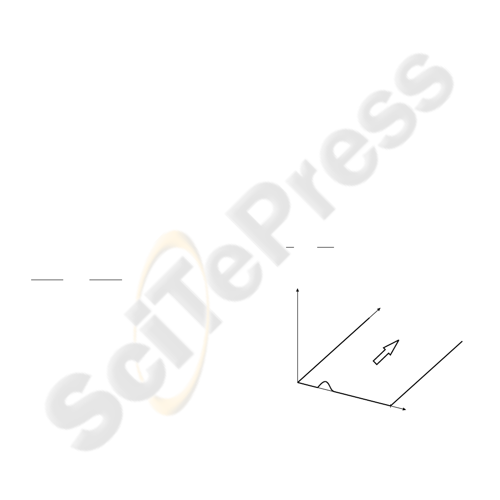
vector of control inputs u. The illustration of PDE (1)
is given on Figure 1 below.
t
x
t
initial condition
time evolution
space variable
right
boundary condition
left
boundary condition
a
Figure 1: Illustrative scheme of the system (1)
The PDEs (1) are used extensively to model and
control chemical processes. For details see (Panagio-
tis, 2001).
281
Cichy B., Gałkowski K., Gramacki A., Gramacki J. and Jank G. (2004).
STABILITY ANALYSIS AND SIMULATIONS OF A CLASS OF CONTINUOUS LINEAR 2D SYSTEMS.
In Proceedings of the First International Conference on Informatics in Control, Automation and Robotics, pages 282-287
Copyright
c
SciTePress

From the system theory point of view, such a sys-
tem can be considered as a singular 2D system as
there is no the term
∂
2
x(t,τ )
∂τ ∂t
in (1). This yields that
the standard methods used in such a case for stability
analysis and stabilization cannot be used directly and
must be reconsidered.
The aim of this paper is to introduce a new physi-
cally motivated stability notion, and show preliminary
developments in LMI based stability tests and state
feedback controller design for this system class. It is
to note that LMI techniques are the new, optimization
based, very efficient numerically methods, recently
extensively used for solving numerous difficult stabil-
ity related problems, for details see e.g. (S. Boyd and
Balakrishnan, 1994). Also a Matlab simulation tool
for the processes of this class has been constructed
and has been briefly shown.
2 STABILITY ANALYSIS BY
USING LMI METHODS
Define Lyapunov function of the form
V (x, t, τ ) = x
T
(t, τ)P x(t, τ) (4)
where P is an appropriately dimensioned symmet-
ric positive definite matrix. This enables introducing
the following stability definition, which can be easily
handled by Lyapunov based techniques.
Definition 1 (Bidirectional stability) The system of
(1) is called bidirectionally stable if and only if is
asymptotically stable in both directions t and τ for
each possible value of the derivative
∂x(t,τ )
∂τ
and
∂x(t,τ )
∂t
respectively, i.e. there exists such a Lyapunov
function of the form (4) that satisfies
∂V (x)
∂t
< 0, ∀x(t, τ),
∂x(t, τ)
∂τ
(5)
∂V (x)
∂τ
< 0, ∀x(t, τ),
∂x(t, τ)
∂t
(6)
The following LMI based necessary and sufficient
condition for the bidirectional stability can be now de-
veloped.
Theorem 1 The system (1) is bidirectionally stable if,
and only if, ∃P
1
> 0 and W > 0, that following LMIs
are feasible.
·
A
T
2
P
1
+ P
1
A
2
−P
1
A
1
−A
T
1
P
1
0
¸
≤ 0 (7)
·
A
1
W A
T
2
+ A
2
W A
T
1
−I
−I 0
¸
≤ 0 (8)
Proof: First consider the condition (5) and rewrite
(1) in the form
∂x
∂t
= −A
1
∂x
∂τ
+ A
2
x (9)
Note that
˙
V (x) = ˙x
T
P x + x
T
P ˙x
= −
∂x
∂τ
T
A
T
1
P x + x
T
A
T
2
P x
− x
T
P A
1
∂x
∂τ
(10)
which combined with (9) gives us the requirement
that ∃P
1
> 0 that following LMI is feasible
·
A
T
2
P
1
+ P
1
A
2
−P
1
A
1
−A
T
1
P
1
0
¸
≤ 0 (11)
In what follows, consider (6). Now (1) can be rewrit-
ten as
∂x
∂τ
= −A
−1
1
∂x
∂t
+ A
−1
1
A
2
x (12)
and it is straightforward to see that (6) holds if ∃
a P
2
> 0 that following LMI is feasible
·
(A
−1
1
A
2
)
T
P
2
+ P
2
(A
−1
1
A
2
) −P
2
A
−1
1
−A
−T
1
P
2
0
¸
≤ 0
(13)
which can be simplified to the form
·
A
T
2
A
−T
1
P
2
+ P
2
A
−1
1
A
2
−P
2
A
−1
1
−A
−T
1
P
2
0
¸
≤ 0 (14)
and left and right multiply (14) by diag{P
−1
2
, I} to
obtain
·
P
−1
2
A
T
2
A
−T
1
+ A
−1
1
A
2
P
−1
2
−A
−1
1
−A
−T
1
0
¸
≤ 0
(15)
Next left and right multiply this result by diag{A
1
, I}
and substitute P
−1
2
b=W to obtain
·
A
1
W A
T
2
+ A
2
W A
T
1
−I
I 0
¸
≤ 0 (16)
only if ∃ a W > 0.
Note however that the test of Theorem 1 cannot be
efficiently handled by LMI solvers due to the presence
of zero blocks (2,2) in both LMIs and the presence of
nonstrict inequalities, which also makes the solution
more difficult. Instead, we propose the following ap-
proach.
Theorem 2 The system (1) is bidirectionally stable if
∃P
1
> 0, W > 0 such that the following LMIs are
feasible
·
A
T
2
P
1
+ P
1
A
2
−P
1
A
1
−A
T
1
P
1
−²I
¸
≤ 0 (17)
·
A
1
W A
T
2
+ A
2
W A
T
1
−I
−I −²I
¸
≤ 0 (18)
for 0 < ² ¿ 1.

Proof: Proof is immediate when noting that LMIs
of (7)–(8) are the limit cases of (17)–(18) where
² → 0.
The test of the Theorem 2 can be performed effi-
ciently by minimizing ² > 0 subject to LMIs (17)–
(18). If such an ² is close to zero, the process is stable.
3 STATE FEEDBACK
STABILIZATION BY USING
LMI
Consider a closed loop control law of the standard
form
u(t, τ) = Kx(t, τ ) (19)
Our aim now is to find a matrix K such that the re-
sulted closed loop system is bidirectionally stable, i.e.
∃P
1
> 0 and W > 0 such that the following matrix
inequalities hold
·
(A
2
+ BK)
T
P
1
+ P
1
(A
2
+ BK) −P
1
A
1
−A
T
1
P
1
−²I
¸
≤ 0
(20)
·
A
1
W (A
2
+ BK)
T
+ (A
2
+ BK)W A
T
1
−I
−I −²I
¸
≤ 0
(21)
for 0 < ² ¿ 1. However, this result is not in the LMI
form and cannot serve as an efficient design tool. But,
it is a base for the following main result.
Theorem 3 The system (1) is bidirectionally stable
under the control low of (19) when ∃W > 0 and N ,
such that the following LMIs are feasible
·
A
2
W + W A
T
2
+ BN + N
T
B
T
−A
1
−A
T
1
−²I
¸
≤ 0 (22)
·
A
1
W A
T
2
+ A
2
W A
T
1
+ A
1
N
T
B
T
+ BN A
T
1
−I
−I
−²I
¸
≤ 0 (23)
for 0 < ² ¿ 1 and then the controller matrix K of
(19) is obtained as
K = N W
−1
(24)
Proof: First, left and right multiply (20) by
diag{P
−1
1
, I} to obtain
·
P
−1
1
(A
2
+ BK)
T
+ (A
2
+ BK)P
−1
1
−A
1
−A
T
1
−²I
¸
≤ 0
Assume now that P
−1
1
≡ W then we have
·
W (A
2
+ BK)
T
+ (A
2
+ BK)W −A
1
−A
T
1
−²I
¸
≤ 0
Assume also KW = N to obtain (22). Next, substi-
tute KW = N to (21) to obtain immediately (23)
what finished our proof. Consider that, stabiliza-
tion requires common solution W for both LMIs. In
(K. Galkowski and Owens, 2002) one can see a sim-
ilar approach of using LMI technic in control prob-
lems.
Consider an unstable example of (1) with following
system matrices
A
1
=
·
−0.09 −0.87
1.48 −0.26
¸
, A
2
=
·
1.70 −0.10
0.19 −1.69
¸
B =
·
−0.71 −0.90
0.21 1.24
¸
The LMIs of Theorem 3 are feasible and the controller
matrix K defined by (24) is now
K =
·
421.8 98.16
−174.1 −268.2
¸
4 NUMERICAL SIMULATIONS
Now we solve numerically and simulate the dynam-
ics of the system of (1) with given boundary condi-
tions (2) and initial condition (3). Hence consider the
following model with two states x
1
and x
2
and three
inputs u
1
, u
2
and u
3
with model matrices as below
A
1
=
·
0.7 −0.1
0.2 −0.1
¸
A
2
=
·
−0.5 0.6
0.7 −1.3
¸
B =
·
1 0.2 −0.3
0.1 0.2 0.3
¸
(25)
We consider the solution on the following mesh
- ’spatial’ direction τ : 60 equally spaced points in
0 ≤ τ ≤ 2π = α; ’time’ direction t: 40 equally
spaced points in 0 ≤ t ≤ 15. For illustrative pur-
poses we also show the built-in property of the solver
i.e we double the number of spatial mesh points in the
second half of the space variable τ.
Initial and boundary conditions must also be sup-
plied. Hence we assume four boundary conditions
x
1
(t, 0) = 0.4
x
1
(t, 2π) = 0
x
2
(t, 0) = −0.2
x
2
(t, 2π) = 0 (26)
and two initial conditions
x
1
(0, τ) = e
−5(τ −1)
2
x
2
(0, τ) = sin(τ ) (27)
We act for the system with three different sets of in-
puts
Set #1
"
u
1
u
2
u
3
#
=
"
0
0
0
#
(28)

Set #2
"
u
1
u
2
u
3
#
=
"
0
0
0
#
for τ > 2
"
u
1
u
2
u
3
#
=
"
−0.3
−0.2
−0.1
#
for τ ≤ 2 (29)
Set #3 where control values depend on t
"
u
1
u
2
u
3
#
=
"
0
e
−t
0
#
(30)
To obtain a numerical solution, a MATLAB’s PDE
solver pdepe is used - see (MathWorks, 2002) for
details. It solves a class of parabolic/eliptic partial dif-
ferential equation (PDE) systems. The general class
to which pdepe applies has the form
c
µ
τ, t, x,
∂x
∂τ
∂x
∂t
= x
−m
∂
∂τ
µ
x
m
f
µ
τ, t, x,
∂x
∂τ
¶¶
+ s
µ
τ, t, x,
∂x
∂τ
(31)
where in our case 0 ≤ τ ≤ 2π and 0 ≤ t ≤ 15.
The integer m = 0 see (MathWorks, 2002) for de-
tails. The (in general) function c is a diagonal matrix
and the flux and source functions f and s are vector
valued. Initial and boundary conditions must be sup-
plied in the following form. For 0 ≤ τ ≤ 2π and
t = 0 the solution must satisfy x(t, 0) = x
0
(t) for a
specified function x
0
. For τ = 0 and 0 ≤ t ≤ 15 the
solution must satisfy
p
l
(τ, t, x) + q
l
(τ, t)f
µ
τ, t, x,
∂x
∂τ
= 0 (32)
for specified functions p
l
and q
l
. Similarly for τ = 2π
and 0 ≤ t ≤ 15,
p
r
(τ, t, x) + q
r
(τ, t)f
µ
τ, t, x,
∂x
∂τ
= 0 (33)
must hold for specified functions p
r
and q
r
. Below
there is a source code used in simulation of the exam-
ple (25) in the form expected by pdepe with the third
set of control inputs (30).
function [x1, x2] = cont2D
m = 0;
alpha = 2*pi;
% values at which the numerical solution is computed
% mesh points
tau = [linspace(0, alpha/2, 20)
linspace(alpha/2+0.1, alpha, 40)]; % spatial variable
t = linspace(0, 15, 40); % time variable
u = [0; 0; 0];
sol = pdepe(m,@pdefun,@pdeic,@pdebc,tau,t,[],u);
x1 = sol(:,:,1)
x2 = sol(:,:,2);
% A surface plot is often a good way to study a solution.
figure;
surf(tau, t, x1);
title(’component x_1’,’FontSize’, 12);
xlabel(’space variable tau’,’FontSize’, 12);
ylabel(’time variable t’,’FontSize’, 12);
figure;
surf(tau, t, x2);
title(’component x_2’,’FontSize’, 12);
xlabel(’space variable tau’,’FontSize’, 12)
ylabel(’time variable t’,’FontSize’, 12);
% --------------------------------------------
function [c,f,s] = pdefun(tau,t,x,DxDtau,u)
c = [1;1];
f = [0;0];
A1 = [0.7, -0.1; 0.2, -0.1];
A2 = [-0.5, 0.6; 0.7, -1.3];
B = [1, 0.2, -0.3; 0.1, 0.2, 0.3];
s = -A1*DxDtau + A2*x + B*[0; exp(-t); 0];
% --------------------------------------------
function u0 = pdeic(tau,u)
u0 = [exp(-5*(tau-1).ˆ2); sin(tau)];
% --------------------------------------------
function [pl,ql,pr,qr] = pdebc(xl,ul,xr,ur,t,u)
pl = [ul(1)-0.4; ul(2)+0.2];
ql = [0; 0];
pr = [ur(1); ur(2)];
qr = [0; 0];
The algorithm implemented in pdepe is as follow.
The routine uses a second-order spatial discretization
method based on mesh values of the spatial variable
τ. Hence the choice of them has strong influence on
the accuracy and cost of computations. The integra-
tion in time variable t is performed using ode15s
solver and hence the timestep is chosen dynamically
(MathWorks, 2002). The time t values are used only
as points where the solution is returned (and printed)
and hence have little impact on the accuracy and cost
of computations.
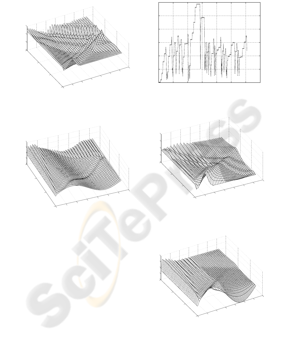
For example to produce Figure 5, Matlab has per-
formed calculations in 305 time points compared with
40 ones chosen by the user for plot the result of calcu-
lations. Number 305 has been obtained by analyzing
the time variable t inside the function pdefun() in
0
1
2
3
4
5
6
7
0
5
10
15
−2
−1
0
1
space variable tau
component x
1
time variable t
Figure 2: The resulting plot of x
1
(t, τ ) with control inputs
(29)
0
1
2
3
4
5
6
7
0
5
10
15
−2
−1
0
1
2
space variable tau
component x
2
time variable t
Figure 3: The resulting plot of x
2
(t, τ ) with control inputs
(29)
the source code above. Figure 4 shows the relation-
ship between 305 calculation points in the time vari-
able and the timestep values chosen dynamically by
the solver.
Notice also that the call to pdepe above includes
the input argument [ ] as a placeholder for additional
argument u. The place with [] is reserved for ad-
ditional options for ode15s (see Matlab’s help of
odeset function) which are not used in our case.
Moreover the parameter u must be passed to each of
the remaining subfunctions even if it is not used there
directly.
The resulting plots of x
1
(t, τ) and x
2
(t, τ) with the
second set of control inputs (29) i.e. with step control
are given on Figures 2 and 3.
The resulting plots of x
1
(t, τ) and x
2
(t, τ) with the
third set of control inputs (30) and partially doubled
spatial mesh points as described at the beginning of
0 50 100 150 200 250 300 350
0
0.02
0.04
0.06
0.08
0.1
0.12
calculation points
timestep values chosen by the solver
Figure 4: Timestep dynamically chosen by the solver
0
1
2
3
4
5
6
7
0
5
10
15
−0.5
0
0.5
1
1.5
space variable tau
component x
1
time variable t
Figure 5: The resulting plot of x
1
(t, τ ) with control inputs
(30)
0
1
2
3
4
5
6
7
0
5
10
15
−1
−0.5
0
0.5
1
space variable tau
component x
2
time variable t
Figure 6: The resulting plot of x
2
(t, τ ) with control inputs
(30)

this section are given on Figures 5 and 6. The waves,
due to constant left and right boundary conditions ”re-
flects” from this boundaries and finally they turn out
even despite of existence of control (it exponentially
decrease in time).
5 CONCLUSIONS AND FURTHER
WORK
In the paper, the preliminary results on stability and
stabilization for a class of singular 2D linear continu-
ous systems has been presented. Also the simulation
tool has been developed. Numerical examples show
that the stabilisation methods performed here are as-
sociated with the comparably high value /energy/ con-
trol which can be troublesome. The solution for it
can be the guaranteed cost control methods, which
is aimed to be the future research topic in this area.
Also, the problems with incomplete model informa-
tion are very important in all practical cases and can
be relatively easily solved by LMI techniques.
REFERENCES
K. Galkowski, E. Rogers, S. X. J. L. and Owens, D. H.
(2002). LMIs – a fundamental tool in analysis and
controller design for discrete linear repetitive pro-
cesses. IEEE Transactions on Circuits and Systems.
MathWorks, T. (2002). Using MATLAB, Inc. USA.
Panagiotis, D. P. C. D. (2001). Nonlinear and Robust Con-
trol of PDE Systems: Methods and Applications to
Transport-Reaction Processes. Birkhauser Boston.
S. Boyd, L. E. Ghaoui, E. F. and Balakrishnan, V. (1994).
Linear Matrix Inequalities in Systems and Control
Theory. SIAM, Philadelphia.
