
AUTONOMOUS NAVIGATION ROBOTIC SYSTEM TO
RECOGNIZE IRREGULAR PATTERNS
Danny Dos Santos, Rafael Peñalver and Wílmer Pereira
Grupo de Investigación en Inteligencia Artificial y Robótica, Universidad Católica Andrés Bello,
Urb. Montalbán, Caracas, Venezuela
Keywords: Autonomous Mobile Robots, Learning Algorithms, Artificial intelligence.
Abstract: This paper presents an approximation of navigation problem under unknown environment using
reinforcement learning. The motivation is to represent a robot that can move in a world with streets and
intersections. Each intersection has a different quantity of streets (irregular blocks). The selected algorithms
were Q-Learning and Value Iteration. The robot was programmed only with Q-Learning and we developed
a simulation with both of them. This simulation allows making comparisons in order to determinate in
which situation each algorithm is appropriate.
1 SYNOPSIS
This paper presents a particular application for
unknown environment using two techniques of
reinforcement learning. These algorithms allow an
autonomous agent or robot, to reach a goal by
learning the environment. In our case, the world is
formed by blocks of irregular geometric forms. The
robot does not know a priori the world but he learns
to identify it. The robot only knows previously the
location of the goal, given in terms of coordinates (x,
y).
The reinforcement learning algorithm selected
for the robot was Q-Learning. This algorithm
consists on rewarding or penalizing each possible
action that the robot executes when it interacts with
their environment. This interaction allows the agent,
based on sensor inputs, chooses an action to be
carried out in the world. Besides, given a policy, the
robot is able to reach a goal, learning by trying and
testing.
The simulation was developed using Q-Learning
and Value Iteration in order to test these algorithms
in different worlds. It allows comparing them under
different situations, either changing the form of the
blocks of the world, or changing the position of the
goal.
The robot was built with a Lego Mindstorm 2.0
kit with two light sensors and one rotation sensor.
The selected language for robot application was Java
under Lejos platform and the simulation was
developed in Visual Basic.
2 REINFORCEMENT LEARNING
The reinforcement learning uses recompenses and
penalizations when the agent executes an action in
order to reach the goal. The learned behavior
contains the robot's implicit world model. By using
reinforcement learning it is not needed to have
examples to build and to validate the behavior (like
supervised learning). The behavior is synthesized
using a scalar (reinforcement) as the only source of
information. This information allows evaluate the
action. The agent receives positive, negative or null
reinforcements according situations and action
selected. There is not separation between the
learning phase and the using phase.
In this work, the world is inaccessible a priori to
the robot (it must learn the world), recompenses are
received in any state or situation, and the robot is a
passive apprentice (it does not alter the world).
2.1 The reinforcement and value
functions
In reinforcement learning must be defined a
reinforcement function. This is a function of the
future reinforcements that the agent searches to
maximize. In other words, a relationship exists
between the couple state/action with the
reinforcements. After carrying out an action in a
state, the agent will receive some reinforcement
(reward) given as a scalar value. This reinforcement
defines the value function. The agent learns how to
maximize the sum of the received reinforcements
295
Dos Santos D., Peñalver R. and Pereira W. (2004).
AUTONOMOUS NAVIGATION ROBOTIC SYSTEM TO RECOGNIZE IRREGULAR PATTERNS.
In Proceedings of the First International Conference on Informatics in Control, Automation and Robotics, pages 295-301
DOI: 10.5220/0001145902950301
Copyright
c
SciTePress
when begins from an initial state and proceeds to a
terminal state.
The value function is based on a field of the
mathematics called dynamic programming. To
explain it, some notations is needed: V(x
t
) is an
approximation of the function value in x
t
state; is
the discount factor in the range of [0,1] that causes
that the immediate reinforcement has more
importance than the future reinforcement and
r(x
t
) is
the reinforcement in this state. The value of the state x
t
follow a policy that is the sum of the reinforcements
when it begins of the state x
t
and carrying out good
actions until a terminal state is reached. A simple
relationship exists between the values of the
successive states x
t
and x
t+1
expressed by the
Bellman equation (1):
V(x
t
) = r(x
t
) + V(x
t+1
) (1)
The process of the learning is the process to find
a solution for the equation (1) for all the states x
t
,
through the space of states.
2.2 Value Iteration
One can find an approximation to optimal value
function evaluating for all possible state since x
t
. In
equation (2), u is the action performed in state x
t
and
cause a transition to state x
t+1
and r(x
t
,u) is the
reinforcement received when performing action u in
state x
t
.
V(x
t
) = max
u
(r(x
t
,u) + V(x
t+1
)) (2)
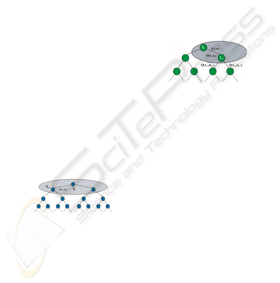
The figure 1 illustrates this process.
Figure 1: Tree of states for Value Iteration
The previous figure describes how update the
value in x
t
. Specifically, there are two possible
actions in the state x
t
, and each one of these actions
directs to different states successors x
t+1
. To update
in Value Iteration, it should find the action that
returns the maximum value (BFS algorithm). The
only way to achieve this is by executing an action
and calculating the sum of the received
reinforcement and the approximate value of the state
successor x
t
.
2.3 Q-Learning
Q-Learning is another extension to the traditional
dynamic programming that solves the problem more
simply. Q-Learning differs from Value Iteration in
that it does not require in a given state each action be
performed and the expected values of the successor
state be calculated. While Value Iteration executes
BFS, Q-Learning takes a single step sample. It only
needs to be the maximum value in the new state to
have all the necessary information to revise the
prediction associated with the executed action. Q-
Learning does not require to calculate on all the
possible successor states. This process is
demonstrated in figure 2:
Figure 2: Tree of States vs. Actions
In Q-Learning each situation-action has a value
(called Q-value). In each state, there is a Q-value
associated with each action (a matrix). The
definition of the Q-value is the sum of the received
reinforcements when the action is executed
following a policy.
The Q-value of a state should approximate the
maximum Q-value in the given state. In this case, it
is easy to derive the equivalent of the Bellman
equation (3) for Q-Learning:
Q(x
t
,u
t
) = r(x
t
,u
t
)+ γ max
ut+1
(Q(x
t+1
,u
t+1
)) (3)
2.3.1 Q-Learning Algorithm
In this application, the algorithm was modified
including ß factor. β represents the learning rate and
it should be bigger than 0. The algorithm steps are:
1. Initialization of the robot's memory: for all the
situation-action couples, the Q-values are zero. It
also could be initialized with random values.
2. repeat
a. x is the situation of the world.
b. The evaluation function selects the action to be
executed: x = Max(Q(x,u'))
where u' represents any possible action. The
selection process depends on the distance to the
goal.
ICINCO 2004 - ROBOTICS AND AUTOMATION
296
c. The robot executes the action u in the world. Be
r the recompense (r can be 0) associated with
the execution of that action in the world.
d. Updates the robot's memory:
Q
t+1
(x,u) = Q
t
(x,u) + ß (r + γ max(Q
t
(x', u')) - Q
t
(x,u))
where x' is the new situation after having been
executed the action in the situation x, u'
represents any possible action.
This algorithm was implemented in Java: LejOS
(Lego Java Operating System) and is executed by
the robot when it navigates in the world.
3 APPLICATION DEVELOPPED
3.1 Design
It should be convenient to design and to prove
different types of physic structures for the
autonomous entity (robot), in order to define and to
build the environment and finally to adjust the
algorithms Q-Learning and Value Iteration.
3.1.1 Robot Design
The accuracy of the movements and the turns are
important, since the robot should make turns on his
owns axis and movements along the streets or roads.
If errors are present in the turn, the robot takes a
wrong road, harming in a significant way the
execution of the algorithm.
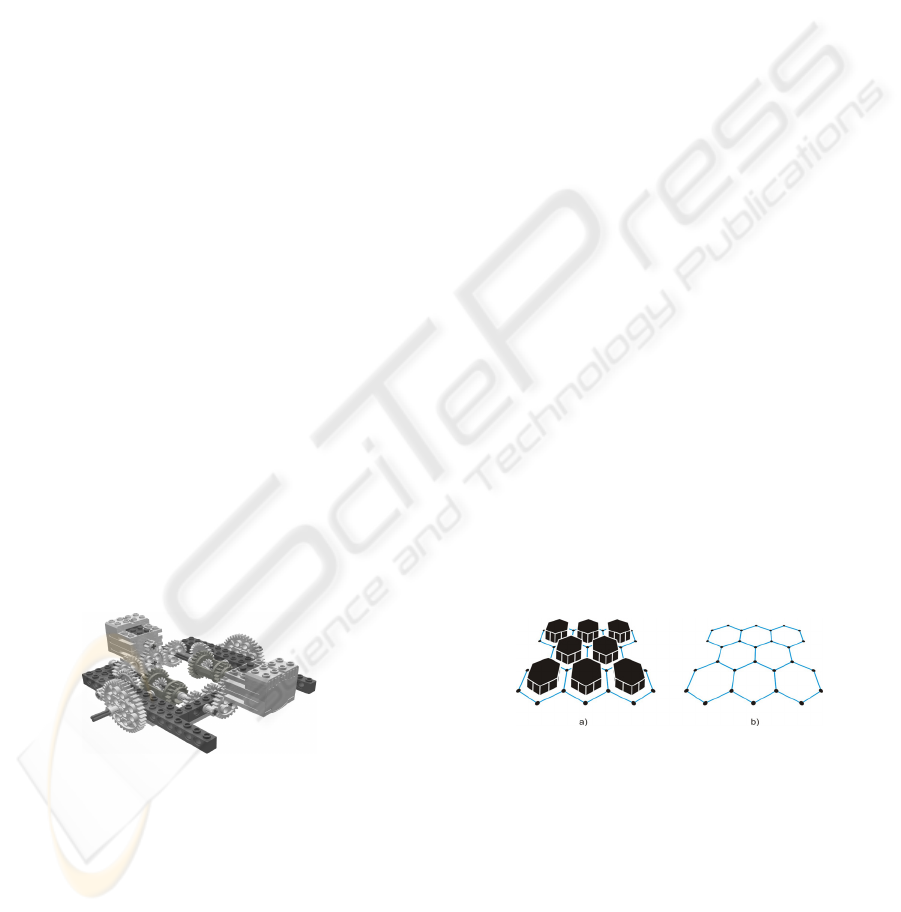
Due to the inaccuracy in the movement, we used
a dual differential drive, such as it shown in the
figure 3.
Figure 3: Transmission system with dual differential
drive
In this system, a motor takes charge of moving
the robot straight line (forward or back), while the
second motor takes charge of carrying out the turns
(toward the left or toward the right), and one of the
motors should only work at the same time, both
cannot work at the same time. The advantage of
using this system resides in that both wheels work to
the same speed maintaining a uniform movement.
After we made the decision of using two wheels
behind and a stabilizer piece in front of the robot.
This piece acts as a ski, minimizing the close contact
with the floor and achieving a stable movement as
much in the turns as in the right movements.
In order to capture the events of the environment,
a study was made to define what kind of sensors
would be used for such an end. Initially it was
planned to use three ultrasonic sensors, placed one in
the robot's front part, and the other ones two in the
lateral sides of the same one. However, serious
inconveniences arose since with the sensors the
readings, in many cases, they didn't reflect the real
situation, for example, when it happens a
phenomenon called speculate reflection.
It was adopted two sensor of light under the
robot pointing toward the floor and a rotation sensor.
This solves part of the problems mentioned
previously, as the recognition of roads and
intersections. The sensor of light maintains adjusted
the robot to the road because that, if the road is of a
certain color, for example blue, and then it detects
another color, for example white, is adjusted to
follow the road. The rotation sensor allows to know
how many degrees the robot has rotated, being an
important element for the robot's navigation. It could
obtain an error of ±10º.
Finally the last sensor of light was placed
pointing to the floor in the robot's front part, which
allows to detect in a quick and simple way how
many roads are in each intersection.
3.1.2 Environment
With the elimination of the sonar, we decided to
eliminate the walls and to identify background, roads
and intersections with the white, blue and black
color, respectively.
Figure 4: World types. a) With walls. b) Without walls
3.1.3 Q-Learning adaptation
Firstly, it is necessary to learn how to arrive to a
specific point of the map from a beginning point. In
each intersection it should be decided among a series
of roads, some move away the robot of the goal,
other brings near it and some even maintain the same
distance from the goal. If an action in that state
brings near the robot of the goal, this action it should
be rewarded, while if the robot goes away, the action
AUTONOMOUS NAVIGATION ROBOTIC SYSTEM TO RECOGNIZE IRREGULAR PATTERNS
297
should be penalized. The autonomous entity should
learn how to arrive to its destination choosing the
actions that offer a bigger recompense.
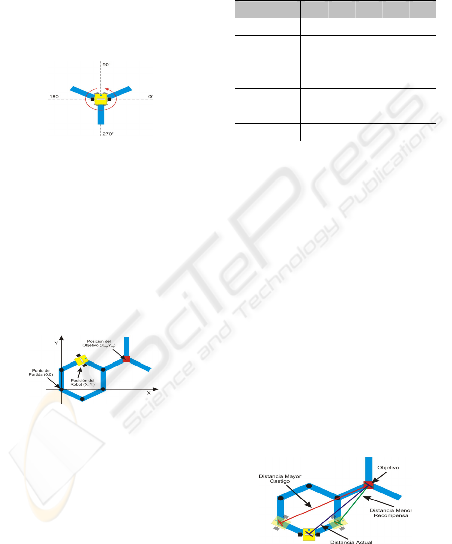
Q-Learning requires to elaborate a matrix
(mainly called Q-Matrix) of actions against states.
The actions in this case are: rotate a specific angle
and to move straight . The figure 5 shows some of
the possible actions that the robot can take in an
intersection with three ways:
Figure 5: Actions that the robot can carry out in an
intersection type
In the Q-Matrix, these actions are denominated
by the value of the angle that should be rotated.
The states represent situations that can happen in
the robot's interaction with the world and they can be
directly the values read by the sensors, combinations
or derived abstractions of the readings of the sensors
or robot's internal representations.
The proposed design of states was one where the
robot built a coordinated system where the origin is
the starting point (Figure 6) and the coordinates of
the goal are already fixed and known previously by
the robot. Using these references, and trigonometric
calculations, the distance is calculated between the
robot and the goal or objective.
Figure 6: System of coordinates used by the robot
It is also necessary to know where is the robot
with respect to the goal (if it is above, below, to the
right or to the left of the goal). To obtain that
information, the coordinates of the goal are
subtracted with the robot's coordinates, for example,
if the subtraction of the abscissas and the coordinates
are negative, the robot is above and to the left of the
goal. The combinations between the quadrants and
the differences among the distances from the robot
to the goal define seven states.
The Q-Matrix (table 1) was built using the states
mentioned previously, and they took the actions as
the angles from 0° up to 360° numbered of 10 in 10
(rotation sensor precision), that is to say, 0°, 10°,
20°, etc. The lines are the states and the columns are
the actions.
Table 1. Q-matrix
State\Action 0 10 ....... 350 360
0 0,48 1 ....... 0,93 0,23
1 0,70 0,60 ....... 0,67 0,37
2 0,97 0,45 ....... 0,23 0,87
3 0,65 0,74 ....... 0,62 0,34
4 0,10 0,76 ....... 0,34 0,73
5 0,29 0,56 ....... 0,89 0,66
6 0,69 0,77 ....... 0,83 0,65
Each state has associated a series of angles that
represent the possible actions. For example, if the
robot arrived to an intersection that brought near it to
the objective and it is in the quadrant 3, the state that
represents this action is the state 5. Once identified
the state, determines the action that it will take
looking for the biggest value in the line for that state.
In the table 1, it can be appreciated that the
maximum value for the state 5 corresponds to the
angle of 350° for what the action that the robot will
take will be the one of rotating up to 350° to move
later on straight line until the next intersection.
These value used to determine the maximum, Q-
values, represent the utility of a couple (state/action).
Once done this and coming to the following
intersection, the robot identifies the state again. It
calculates the recompense of the action taken in the
previous state. A positive recompense takes place
when the robot executes an action that brings near it
to the goal, rewarding it. While a negative
recompense takes place when instead of coming
closer to the goal this goes away, for what the
executed action is penalized (figure 7). With the
calculated recompense, the Q-value is updated
(value in the Q-Matrix) corresponding to the couple
(previous state-action) modifying the values that can
affect to future decisions for that state.
Figure 7: Rewards of the possible actions that the
robot can take
ICINCO 2004 - ROBOTICS AND AUTOMATION
298
3.2 Tests
In this last phase was carried out successive tests for
the detection of error. The robot's acting was
observed in the environment and the behavior of the
algorithm Q-learning applied for the navigation.
Nevertheless, the principal objective in this
phase is to establish the comparisons among Value
Iteration and Q-Learning, using the simulation. It is
important to mention that a iteration begins with the
robot in the starting point and it concludes when this
arrives to the goal. Each run can have associated a
finite number of iterations.
With regard to the simulation, the algorithms Q-
Learning and Value Iteration, one could observe the
behavior of each one in an ideal world. In this way,
we can carry out comparisons between both
algorithms, avoiding the problems with the
inaccurate of the sensors. Also, modifications can be
made in certain parts of the algorithms, without
altering the logic of them.
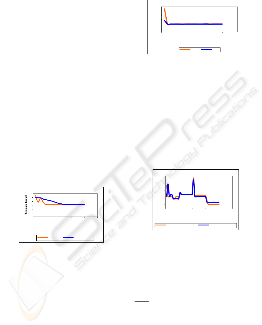
Test 1
There was carried out a run of 20 iterations,
maintaining the goal fixes, with each one of the two
algorithms to see how it was the learning curve in
both cases. The obtained graph was the following
one:
0
1
2
3
4
5
6
0 5 10 15 20 25
Iter aciones
Q-Lear ning Value Iter ation
Figure 8: Learning curves of Q-Learning and Value
Iteration
Here one can observe that Q-Learning converges
in quicker way than Value Iteration, that is to say, it
takes less learning time to arrive to the goal. Even
though Value Iteration takes more time to learn, both
of them find efficiently the goal with the movement
policy.
Test 2
Since the Q-Matrix can be initialized with
random values or with values in zero, they were
carried out two runs where one of them was
initialized with random values and the other one
with zeros. The result was the following one:
0
2
4
6
8
10
12
0 5 10 15 20 25
Iteraciones
Tiempo (seg)
Aleatorio Ceros
Figure 9: Learning curves of Q-Learning
You can infer of this graph that don't care values
with which the Q-Matrix is initialized, since always
it will converge in a similar way. The only thing that
could change is the time that takes in learning how
to arrive to the goal in the first iterations.
Test 3
Were carried out 2 runs of the Q-Learning
algorithm of 40 iterations each one, changing the
position of the goal after each 10 iterations and
maintaining it fixed during those 10 iterations. For
the first run we worked with the matrix initialized
with random values and for the second run the
matrix was initialized with zeros. The resulting
graph was the following one:
0
1
2
3
4
5
6
7
8
9
0 1020304050
Iteraciones
Tiempo (seg)
Q-Learning (Matriz Aleatoria) Q-Learning(Matriz Cero)
Figure 10: Learning curve of Q-Learning varying goal
Here we can observe that the behavior of Q-
Learning for both cases is similar, they are able to
almost establish the same time of arrival to the goal.
The peaks represent the point where the goal was
changed position and due to this, the algorithm takes
more time for the learning when trying to adapt to
the new change.
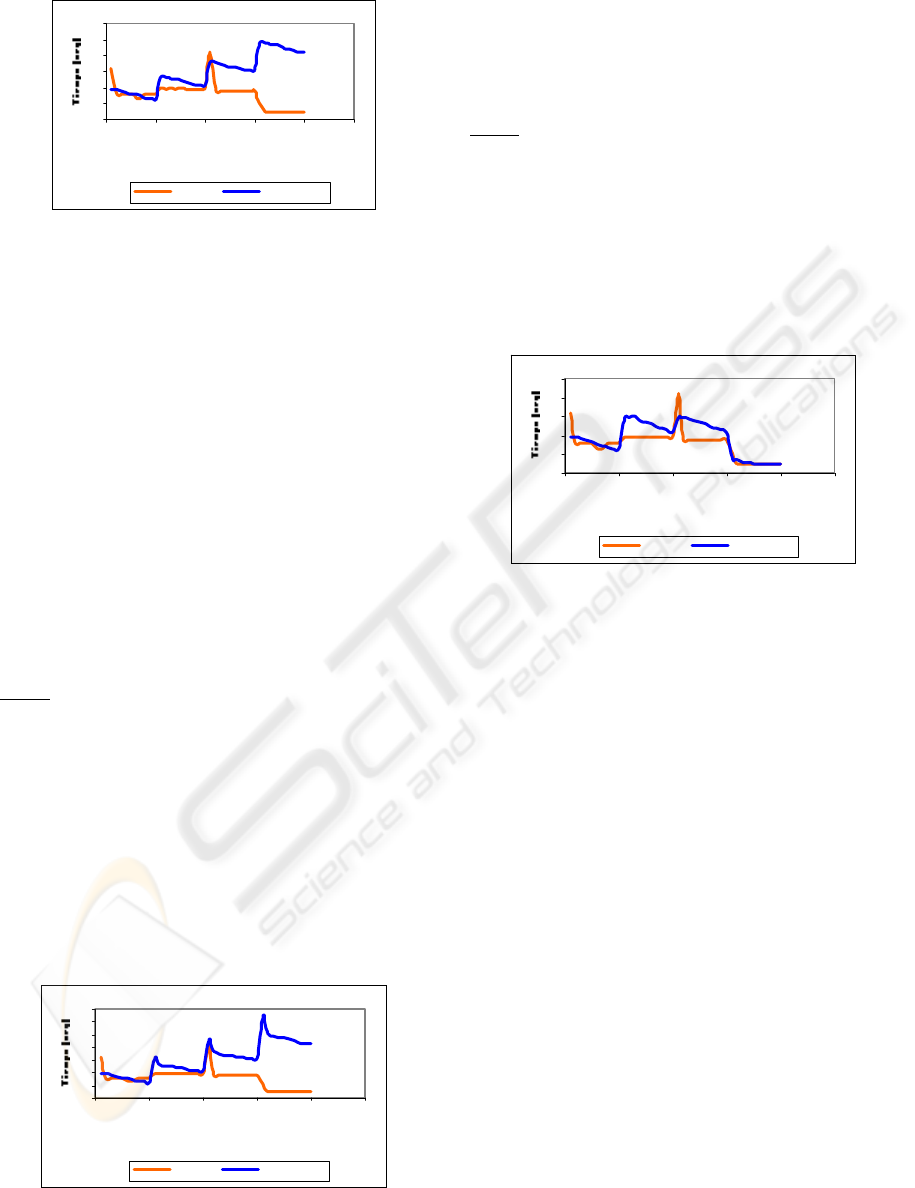
Test 4
Were carried out 2 runs of 40 iterations each one,
changing the position of the goal each 10 iterations.
For the first run we worked with the Q-Learning
algorithm and for second one, the algorithm Value
Iteration. The resulting graph was the following:
AUTONOMOUS NAVIGATION ROBOTIC SYSTEM TO RECOGNIZE IRREGULAR PATTERNS
299
0
2
4
6
8
10
12
0 1020304050
Iter aciones
Q-Lear ni ng Value Iteration
Figure 11: Learning curves of Q-Learning and Value
Iteration varying goal
As you can observe, Q-Learning adapts to the
changes in a quick way and like the previous graph.
However, Value Iteration, once had concluded the
learning of the route to the goal, when it change, the
new time that takes is equivalent at the time that
took in arriving to the position previous of the goal
plus the time that needs learn how to arrive to the
new position of the goal.
It is important to notice that Value Iteration, keep
the route in a state’s graph. It is affected critically if
it is forced to go by a node or intersection already
visited. Each intersection has assigned an action that
was been of the previous learning, what causes to
take the same road every time that arrives to that
state. It does not carried out the learning process for
that intersection, retarding the arrival to the new
position of the goal.
Test 5
Due to the previously exposed problem for the
Value Iteration algorithm and for the time that takes
learning how to arrive to the new goal. It was
decided to make a modification that consisted on
eliminating the condition of learning end, that is to
say that is carried out the learning process in each
node or visited intersection. For this case it were also
carried out 2 runs changing the position goal, of 20
iterations each one, using for the first one the Q-
Learning algorithm and for second one the Value
Iteration algorithm. The resulting graph is shown
next:
0
2
4
6
8
10
12
14
0 1020304050
I ter aci ones
Q-Lear ni ng Value Iteration
Figure 12: Learning curves of Q-Learning and Value
Iteration modified varying goal
We observed that there was not a significant
change in the behavior of Value Iteration, because it
follows the same behavior patterns of the previous
case, only that the learning was made in all moment,
in each intersection visited or not visited.
Test 6
Lastly, there was carried out a second
modification in the Value Iteration algorithm that
consisted in reinitialize the graph every time that the
position of the goal was changed, maintaining the
condition of learning end. Were also carried out 2
runs of 20 iterations each one, changing the position
of the goal and using for the first run the algorithm
Q-Learning and for second one the algorithm Value
Iteration.
0
2
4
6
8
10
0 1020304050
I ter aci ones
Q-Lear ni ng Value Iteration
Figure 13: Learning curves of Q-Learning and Value
Iteration modified varying goal
For this case, the algorithm Valued Iteration
adapted better to the changes of position of the goal,
but that in comparison with Q-Learning, it continues
taking more time of learning than the one used by Q-
Learning. The disadvantage of this is that no longer
keeps its knowledge if the robot should travel the
world again.
It is necessary to highlight that the Value
Iteration algorithm always search the shortest route,
while Q-Learning only tries to arrive to the goal
according to a policy of movements product of the
learning. Occasionally, Value Iteration visited less
intersections than those visited by Q-Learning
4 CONCLUSIONS
Along this work, we studied different aspects of the
artificial intelligence applied to the area of the
learning, specifically the reinforcement learning.
They allow solve a great variety of problems where
learning is an important factor to search a solution.
The use of the kit Lego MindStorm, with LejOS,
was appropriate for the construction of the robot's
prototype, because it allows build easy and quickly a
great variety of adaptive robots' models to diverse
problems. However, a disadvantage of the kit is the
ICINCO 2004 - ROBOTICS AND AUTOMATION
300

quantity of inputs or sensors that has the robot. It
allows connect only three sensors at the same time,
limiting the functionality of the robots and the
complexity of the program that is implemented.
Also, it possesses a limited memory (32Kb), what do
not allow implement very extensive programs. Also,
the firmware, occupies space in the memory,
diminishing even more the capacity to store user's
programs.
The navigation problem to find a goal is possible
to solve using a reinforcement learning algorithm.
Other types of learning techniques exist, as the
evolutionary learning that involves the use of genetic
algorithms and that can be used to solve navigation
problems. These algorithms are slow and they only
allow approximate to sub-optimal solution, without
any guarantee of the convergence to the best
solution. They do not operate on real time execution,
being a restrictive factor for the implementation of
this type of problem.
Value Iteration, as Q-Learning, is based on the
principle of the dynamic programming, which allows
carry out an effective learning through recompenses
and penalizations. The advantage of using Value
Iteration is that the found solution tends to be, in
most of the cases, better than the solution found with
Q-Learning.
The main disadvantage of the Value Iteration
algorithm is that it only can be applied in action-state
schemes where an action taken in a given state, leads
the same successor state. If the goal changes
position, the algorithm takes much more time, since
all the roads that have been taken and then learned
by the robot, these will always be taken even still
when the goal is located in some other point.
With regard to Q-Learning, the main advantages
of using this algorithm are that if the goal changes
position, Q-Learning adjusts its learning efficiently,
being able to always arrive to the goal. Besides if the
Q-Matrix is initialized with random values, the robot
can experience other roads that enlarge his learning.
This is because the algorithm looks always for the
maximum Q-value for all possible actions in a state.
Finally, the learning curve tends to converge in
quicker way that Value Iteration, although in a less
uniform way.
The main disadvantage of using Q-learning is
that the solution found is not always the best one,
although it tends to be very near of it.
In this point one could wonder under what
conditions one of these two reinforcement learning
algorithms should be chosen? The answer comes
given depending on the situation. If the time to
arrive to the goal is not a problem, you can apply
Value Iteration, otherwise Q-Learning is the best
option. However, for both cases, the route that finds
Value Iteration is similar to the route that finds with
Q-Learning, varying very little with respect to the
other one.
When programs are designed based on
reinforcement learning algorithms, it is necessary to
define and to design in a detailed way the states,
actions and the reward policy, since these factors
play a very important role in the operation of the
algorithm. If some of these factors flaw, the acting of
the algorithms can be seriously affected, or worse, it
could not arrive to any solution.
REFERENCES
Bagnall, B. 2002, CORE Lego MindstormsTM
Programming. Edit. Prentice Hall PTR. New York,
United States of America.
Ferrari, G., Gombos, A. Hilmer, S., Stuber, J., Porter, M.,
Waldinger, J. and Laverde, D. 2002, Programming
Lego MindstormsTM with Java. Edit. Sysgress.
United States America.
Russel, S. and Norvig, P. 1996, Artificial Intelligence A
modern approach. First edition. Edit. Prentice Hall,
1996.
Carrasquero Z., Oscar H. and McMaster F., Eduardo 2002,
Design and a robot's construction with the module
RCX 1.0 for not predetermined worlds (Thesis of
Engineer in Computer, Catholic University Andrés
Bello).
Bagnall, Bryan 2001, LejOS: Java for the RCX. [web page
on-line] Consulted in 10/5/2003 Available in
http://lejos.sourceforge.net /.
Dartmouth College Computer Science Department (2001).
Robbery-Rats Locomotion: Dual Differential Drive.
[web page on-line] Consulted in 20/5/2003 Available
in
http://www.cs.dartmouth.edu/~robotlab/robotlab/cour
ses/cs54-2001s/dualdiff.html
Gross M., Stephan V. and Boehme J. 1996, Sensory based
robot navigation using self-organizing networks and
Q-Learning. [document on-line] Consulted in
12/9/2003 Available in
http://citeseer.nj.nec.com/gross96sensorybased.htm
Mance E. Harmon and Stephanie S. Harmon (s.f.).
Reinforcement Learning: A Tutorial. [ document on-
line] Consulted in 20/9/2003 Available in
http://www.nada.kth.se/kurser/kth/2D1432/2003/rltut
orial.pdf.
Touzet, Claude F. 1999, Neural Networks and Q-Learning
for Robotics. [document on-line] Consulted in
3/9/2003 Available in
http://avalon.epm.ornl.gov/~touzetc/Publi/Touzet_IJC
NN_Tut.pdf.
Zou Yi, Ho Yeong Khing, Chua Chin Seng and Zhou Xiao
Wei 2003, Evidence method in ultrasonic sensor
coalition for mobile robots. [document on-line]
Consulted in 10/8/2003 Available in
http://www.duke.edu/~yz21/research/YZ_IASTED-
MIC2000.pdf.
AUTONOMOUS NAVIGATION ROBOTIC SYSTEM TO RECOGNIZE IRREGULAR PATTERNS
301
