
RECURSIVE MOESP TYPE SUBSPACE IDENTIFICATION
ALGORITHM
Catarina J. M. Delgado
Faculdade de Economia do Porto
Rua Dr. Roberto Frias, 4200-464 Porto - Portugal
P. Lopes dos Santos
Faculdade de Engenharia da Universidade do Porto
Rua Dr. Roberto Frias, 4200-465 Porto - Portugal
Keywords:
System Identification, Subspace methods, State-space models, Linear Systems, Parameter estimation.
Abstract:
In this paper two recursive algorithms, based on MOESP type subspace identification, are presented in two
versions. The main idea was to show that we can represent subspace identification methods as sequences of
least squares problems and implement them through sequences of modified Householder algorithms. There-
fore, it is possible to develop iterative algorithms with most of the advantages of this kind of methods, and still
improve the numerical efficiency, in order to deal with real-time applications and minimize the computational
burden.
1 INTRODUCTION
The Subspace Identification algorithms aim to esti-
mate, from measured input / output data sequences
({u
k
} and {y
k
}, respectively), the system described
by:
½
x
k+1
= Ax
k
+ Bu
k
+ Ke
k
y
k
= Cx
k
+ Du
k
+ e
k
(1)
E
£
e
p
e
T
q
¤
= R
e
δ
pq
> 0 (2)
where A ∈ R
n×n
, B ∈ R
n×m
, C ∈ R
l×n
, D ∈
R
l×m
, K ∈ R
n×l
and x
k
∈ R
n
. The sequence
{e
k
} ∈ R
l
is a white noise stochastic process and the
input data sequence is assumed to be a persistently ex-
citing quasi-stationary deterministic sequence(Ljung,
1987).
Most of the past contributions ((Larimore, 1990),
(Moonen et al., 1989), (van Overschee and de Moor,
1996), (Verhaegen, 1994), (Viberg et al., 1991))
are centered in the off-line identification of time-
invariant systems field, by developing non-recursive
algorithms. Even though the on-line identification can
be applied to a wider class of systems (time-variant,
non-linear...), it has been a little forgotten due to its
high computation and storage costs. When a particu-
lar subspace off-line identification algorithm (such as
the algorithm introduced by Van Overschee and De
Moor (van Overschee and de Moor, 1996)) is adapted
to a recursive identification algorithm ((Cho et al.,
1994), (Ljung, 1983), (Gustafsson et al., 1998), (Oku
and Kimura, 2000)), not only the computational bur-
den is reduced, but also the application scope is en-
larged, preserving most of the advantages of this kind
of methods.
This paper is organized as follows: in section 2,
the notation is introduced and, in section 3, two ba-
sic MOESP-type algorithms are described: the PO-
MOESP (Verhaegen, 1994) and the R-MOESP (van
Overschee and de Moor, 1996). Sections 4 and 5 are
dedicated to the main results: section 4 introduces
the 2QR recursive version for the MOESP algorithms
and section 5 the 1QR version. Finally, in section 6,
some simulation results are shown and, in section 7,
the conclusions are presented.
2 NOTATION
We define the following block Hankel matrices, built
with input data:
U
p
=
U
(0)
...
U
(i−1)
, U
p+
=
U
(0)
...
U
(i)
,
U
f
=
U
(i)
...
U
(2i−1)
, U
f−
=
U
(i+1)
...
U
(2i)
where U
(i)
= [
u
i
... u
i+j−1
] ∈ R
m×j
and the
subscripts p and f denote past and future data, respec-
176
Delgado C. and dos Santos P. (2004).
RECURSIVE MOESP TYPE SUBSPACE IDENTIFICATION ALGORITHM.
In Proceedings of the First International Conference on Informatics in Control, Automation and Robotics, pages 176-182
DOI: 10.5220/0001146801760182
Copyright
c
SciTePress

tively. In a similar way, Y
(i)
∈ R
l×j
, Y
p
, Y
p+
, Y
f
and
Y
f−
are block Hankel matrices, built with output data.
With both input and output data we can also define
the block hankel matrices
H
p
=
·
U
p
Y
p
¸
, H
p+
=
·
U
p+
Y
p+
¸
,
HU =
·
H
p
U
f
¸
, H
+
U
−
=
·
H
p+
U
f−
¸
and the orthogonal projection matrices
Z
i
= Y
f
/
HU
= Y
f
Π
HU
Z
i+1
= Y
f
/
H
+
U
−
= Y
f
Π
H
+
U
−
where Π
M
= M
+
M = M
T
¡
MM
T
¢
+
M denotes
the orthogonal projection into the row space of M and
(.)
+
denotes the Moore-Penrose pseudoinverse
Other important matrices are the extended observ-
ability matrix
¡
Γ
i
∈ R
li×n
¢
and the block Toeplitz
matrix
¡
H
d
i
∈ R
li×mi
¢
, built with Markov parame-
ters (Delgado and dos Santos, 2004b).
3 MOESP-TYPE ALGORITHMS
The MOESP algorithms can be described as se-
quences of two main steps (van Overschee and
de Moor, 1996). First, the model order n and a ba-
sis for the column space of Γ
i
are determined:
b
Γ
i
=
U
n
S
1/2
n
, where U
n
and S
n
are given by the Singular
Value Decomposition of Z
i
Π
U
f
⊥
= Z
i
− Z
i
/
Uf
:
Z
i
Π
U
f
⊥
= USV
T
= (3)
= [
U
n
U
n
⊥
]
·
S
n
0 0
0 S
n
⊥
0
¸
×
V
T
n
V
T
n1
⊥
V
T
n2
⊥
= U
n
S
n
V
T
n
+ U
n
⊥
S
n
⊥
V
T
n1
⊥
≈
≈ U
n
S
n
V
T
n
When the measurements are noise corrupted, it may
not be straightforward to distinguish the ”nonzero”
singular values (S
n
) from the ”zero” singular values
(S
n
⊥
). Therefore, a better estimate of the system or-
der is obtained by trying different values and then
comparing the simulation errors (van Overschee and
de Moor, 1996).
In the second main step, the system matrices are es-
timated. There are two approaches to estimate those
matrices: the method introduced by Van Overschee,
with the R-MOESP algorithm (van Overschee and
de Moor, 1996), and the method introduced by Ver-
haegen, with the PO-MOESP algorithm (Verhaegen,
1994).
3.1 R-MOESP Algorithm.
When we know an estimate of Γ
i
, matrices A and C
are obtained by solving the following linear equation,
in a least squares sense (van Overschee and de Moor,
1996):
·
Γ
+
i−1
Z
i+1
Y
(i)
¸
=
·
A
C
K
BD
¸·
Γ
+
i
Z
i
U
f
¸
+ ρ (4)
where Γ
i−1
=
£
I
l(i−1)
0
¤
Γ
i
. The matrix K
BD
is
then used to estimate B and D, since
K
BD
=
·
K
A
K
C
¸
= (5)
=
·
B Γ
+
i−1
H
d
i−1
D 0
¸
−
·
A
C
¸
Γ
+
i
H
d
i
=
=
·
N
1
·
D
B
¸
... N
i
·
D
B
¸ ¸
Lopes dos Santos and Martins de Carvalho (dos
Santos and de Carvalho, 2003) have shown that
K
A
can be written as K
A
= K
p
K
C
=
µ
−A
³
Γ
T
i
Γ
i
´
−1
C
T
K
C
. Therefore, we can work
only with:
K
C(B,D)
=
·
K
p
I
l
¸
+
K
BD
= (6)
=
·
N
C1
·
D
B
¸
... N
Ci
·
D
B
¸ ¸
where
N
C1
= [
I
l
− L
C1
−L
C2
... −L
Ci
] G
i
N
Ck
= [
−L
Ck
... −L
Ci
0
] G
i
(k > 1)
L
A
= [
L
A1
L
A2
... LA
] = AΓ
+
i
L
C
= [
L
C1
L
C2
... L
Ci
] = CΓ
+
i
G
i
=
·
I
l
0
0 Γ
i−1
¸
Equation (6) can be rewritten as:
"
K
C1
...
K
Ci
#
=
"
N
C1
...
N
Ci
#
·
D
B
¸
(7)
and B and D estimated in the least squares sense.
3.2 PO-MOESP Algorithm
Another approach to determine matrices A and C is
to use the shift-invariance structure in Γ
i
(Verhaegen,
1994):
b
C = [
I
l
0
]
b
Γ
i
(8)
b
A = Γ
+
i−1
Γ
i
(9)
RECURSIVE MOESP TYPE SUBSPACE IDENTIFICATION ALGORITHM
177

where Γ
i
=
£
0 I
l(i−1)
¤
b
Γ
i
. These estimates of A
and C are the same as the estimates produced by the
method of Van Overschee and De Moor ((Chiuso and
Picci, 2001), (Delgado and dos Santos, 2004a), (dos
Santos and de Carvalho, 2004)).
Then, matrices B an D can be estimated by linear
regression:
vec(by
k
) = [M
D
M
B
]
·
θ
D
θ
B
¸
(10)
where
M
D
= (u
T
k
⊗ I
l
) (11)
M
B
=
(k−1)
X
t=1
(u
T
t
⊗ CA
k−t−1
) (12)
θ
D
= vec(D) (13)
θ
B
= vec(B) (14)
and by
k
is the simulated output, given by
by
k
= Du
k
+
k−1
X
t=1
CA
k−t−1
Bu
t
= by
Dk
+ by
Bk
(15)
with
vec(by
Dk
) = vec(Du
k
) = (16)
= (u
T
k
⊗ I
l
)vec(D)
vec(by
Bk
) = vec
Ã
k−1
X
t=1
CA
k−t−1
Bu
t
!
(17)
=
k−1
X
t=1
¡
u
T
t
⊗ CA
k−t−1
¢
vec(B)
4 RECURSIVE 2QR APPROACH
4.1 The weighted projection
The estimation of Γ
i
from the singular value decom-
position of Z
i
Π
U
f
⊥
is implemented through the LQ
decomposition of
h
U
f
H
p
i
:
·
U
f
H
p
¸
= LQ
L
= (18)
=
·
L
U
0 0
L
H1
L
H2
0
¸
"
Q
L1
Q
L2
Q
L3
#
where L
U1
∈ R
mi×mi
, L
H1
∈ R
(m+l)i×mi
,
L
H2
∈ R
(m+l)i×(m+l)i
and Q
L1
∈ R
mi×j
, Q
L2
∈
R
(m+l)i×j
, Q
L3
∈ R
(j−(2m+l)i)×j
. Matrices L
U1
and L
H2
are two lower triangular matrices and ma-
trix Q
L
is orthonormal and
Q
L
Q
T
L
= I
j
⇔ Q
Lp
Q
T
Lq
=
½
I, if p = q
0, if p 6= q
(19)
Q
T
L
Q
L
=
3
X
k=1
Q
T
Lk
Q
Lk
= I
j
(20)
From this decomposition,
Π
Uf
= U
T
f
(U
f
U
T
f
)
−1
U
f
= Q
T
L1
Q
L1
(21)
Π
HU
=
£
Q
T
L1
Q
T
L2
¤
·
Q
L1
Q
L2
¸
(22)
Π
U
f
⊥
= I
j
− Π
Uf
=
£
Q
T
L2
Q
T
L3
¤
·
Q
L2
Q
L3
¸
(23)
Π
HU
⊥
= I
j
− Π
HU
= Q
T
L3
Q
L3
(24)
If we consider the least squares problem
Y
f
= [θ
Uf
θ
Hp
]
·
U
f
H
p
¸
(25)
we can rewrite it as
B
Q
L
= [θ
Uf
θ
Hp
]
·
L
U1
0 0
L
H1
L
H2
0
¸
(26)
where B
QL
=
£
B
U
B
H
B
UH
⊥
¤
= Y
f
Q
T
L
.
Then,
Z
i
= Y
f
Π
HU
= [B
U
B
H
]
·
Q
L1
Q
L2
¸
(27)
= B
U
Q
L1
+ B
H
Q
L2
As to the weighted projection, it can be expressed as
Z
i
Π
U
f
⊥
= θ
Hp
H
p
Π
⊥
Uf
= (28)
= [
θ
Uf
θ
Hp
]
·
U
f
H
p
¸
Π
⊥
Uf
=
= Z
i
Π
U
f
⊥
= Z
i
− (Z
i
/U
f
) =
= Z
i
− (Z
i
Q
T
L1
Q
L1
) =
= B
H
Q
L2
In a recursive approach, the dimension of the ma-
trices involved must not depend on the number
of measurements (N = j − 2i + 1) . Since Q
L2
∈
R
(m+l)i×(N−2i+1)
, that could be a problem in the
SVD step. However,
(B
H
Q
L2
) (B
H
Q
L2
)
T
= B
H
B
T
H
(29)
and, if B
H
Q
L2
= USV
T
,
(B
H
Q
L2
) (B
H
Q
L2
)
T
= US
2
U
T
= B
H
B
T
H
(30)
This means that B
H
has the same left singular vec-
tors and the same singular values as Z
i
Π
U
f
⊥
. Since
we only need U
n
and S
n
to determine a basis for
the column space of Γ
i
, we only have to deal with
B
H
∈ R
li×(m+l)i
, in order to estimate Γ
i
.
ICINCO 2004 - SIGNAL PROCESSING, SYSTEMS MODELING AND CONTROL
178

4.2 The system matrices
To estimate matrices A, B, C and D, one must solve
two least squares problems: (4) and (7). In the last
one, both matrices K
C
and N
C
have constant di-
mensions, but in the first one that does not happen.
Therefore, we will implement (4) recursively, using
the LQ decomposition, to avoid this dimension prob-
lem, since the least squares solution of
·
Γ
+
i−1
Z
i+1
Y
(i)
¸
T
=
·
Γ
+
i
Z
i
U
f
¸
T
θ
ACK
(31)
with
θ
ACK
=
·
A K
A
C K
C
¸
T
is the same as the least squares solution of
B
(N)
= Q
T
(N)
·
Γ
+
i−1
Z
i+1
Y
(i)
¸
T
= (32)
=
·
R
(N)
0
¸
θ
ACK
To update R
(N)
and B
(N)
we need the last columns
of Y
(i)
, U
f
, Z
i
and Z
i+1
. The last column of Z
i
is
computed directly from (27) and the last column of
Z
i+1
is computed from
Z
i+1
= Y
f−
Π
H+U−
= (33)
= [
B
U−
B
H+
]
·
Q
L1
(i+1)
Q
L2
(i+1)
¸
where
·
U
f−
H
p
+
¸
= L
(i+1)
Q
L1
(i+1)
Q
L2
(i+1)
Q
L3(i+1)
(34)
B
U
−
= Y
f−
Q
T
L1
(i+1)
(35)
B
H+
= Y
f−
Q
T
L2
(i+1)
(36)
However a problem may here arise, since the rows-
paces considered at the k-th iteration are not quite the
same as in the (k+1)-th iteration. In order to deal with
this we have implemented two options: recursive least
squares with a forgetting factor or the sliding window
technique.
4.3 The modified Householder
algorithm
Since our versions of subspace algorithms are se-
quences of least squares problems implemented
through the QR decomposition (or the similar LQ),
we modified the Householder algorithm for matrix
factorization updating, to updates both B and R, at
once. In fact, we apply the same Householder re-
flection to change both R
(N)
and B
(N)
. As R
(N)
is
already a upper triangular matrix, the QR decompo-
sition of R
(N+1)
is faster to compute, because now
there is only one line to set to zero. Therefore, the
Householder Algorithm can be adapted in order to
modify only two rows of the matrix in each iteration k
(the last row and the k-th one), since the others remain
the same. Another version of this modified algorithm
considers the update of the decomposition matrices
when Nr > 1 rows are added.
4.4 Recursive R-MOESP-2QR
algorithm
1. LQ decomposition and the orthogonal projections
(a) Update the last columns of the block Hankel ma-
trices U and Y
³
φ
U(N +1)
and φ
Y (N+1)
´
.
(b) Update the decompositions (18) and (34). Al-
though L
(N+1)
and B
(N+1)
have one more line,
after the LQ decomposition, this last column of
L
(N+1)
has only zero elements and it can be re-
moved. So, the matrices L
(N+1)
and B
(N+1)
still have the dimensions of L
(N)
and B
(N)
.
(c) Determine z
i
and z
i+1
, the last columns of Z
i
and Z
i+1
, as in (27) and (33).
2. The column space of Γ
i
and Γ
i−1
(a) Determine
b
Γ
i
= U
n
S
1/2
n
, where the system or-
der n is assumed to be known (3) and
B
H(N+1)
= USV
T
= U
n
S
n
V
T
n
(37)
(b) Compute
b
Γ
i−1
=
£
I
l(i−1)
0
¤
b
Γ
i
3. Matrices A, C and K
BD
(a) Update the QR decomposition matrices R
AC(N )
and B
AC(N )
:
·
R
AC(N )
r
T
N+1
¸
= Q
AC(N +1)
·
R
AC(N +1)
0
¸
·
B
AC(N +1)
×
¸
= Q
T
AC(N +1)
·
B
AC(N )
b
T
N+1
¸
where
r
N+1
=
·
b
Γ
+
i
z
i(N+1)
[
0 I
mi
] φ
U(N +1)
¸
b
N+1
=
·
b
Γ
+
i−1
z
i+1(N+1)
[
0 I
li
] φ
Y (N+1)
¸
(b) Solve, in the least squares sense, the problem
B
AC(N +1)
= R
AC(N +1)
θ
AC(N +1)
, where
θ
AC(N +1)
=
"
A
T
(N+1)
C
T
(N+1)
K
T
A(N+1)
K
T
C(N +1)
#
RECURSIVE MOESP TYPE SUBSPACE IDENTIFICATION ALGORITHM
179

4. Matrices B and D
(a) Determine K
C(N +1)
, from K
(N+1)
, and matrix
N
C
, as in (6)
(b) Solve the least squares problem (7) recursively
·
B
K(k−1)
K
Ck
¸
=
·
R
N(k−1)
N
Ck
¸·
D
(k)
B
(k)
¸
4.5 Recursive PO-MOESP-2QR
algorithm
1. LQ decomposition and the orthogonal projections
(a) Update the last columns of the block Hankel ma-
trices U and Y
³
φ
U(N +1)
and φ
Y (N+1)
´
.
(b) Update the decompositions (18) and (34).
2. The column space of Γ
i
,
Γ
i
and Γ
i−1
(a) Determine
b
Γ
i
= U
n
S
1/2
n
, where the system or-
der n is assumed to be known (3) and
B
H(N+1)
= USV
T
= U
n
S
n
V
T
n
(b) Compute
b
Γ
i−1
=
£
I
l(i−1)
0
¤
b
Γ
i
(c) Compute
b
Γ
i
=
£
0 I
l(i−1)
¤
b
Γ
i
3. Matrices A and C
(a) Determine
b
A =
b
Γ
+
i−1
b
Γ
i
(b) Determine
b
C = [
I
l
0
]
b
Γ
i
4. Matrices B and D (”minimum simulation error
method”)
(a) Update the QR decomposition
·
B
BD(N)
Y
BD
¸
=
·
R
BD(N)
X
D
X
B
¸·
θ
D
θ
B
¸
where B
BD(N)
∈ R
m(n+l)×1
, R
BD(N)
∈
R
m(N+l)×m(N+l)
and
X
B
=
k−1
X
t=1
u
T
t
⊗ (CA
k−1−t
) ∈ R
l×mn
X
D
= u
T
k
⊗ I
l
∈ R
l×lm
Y
BD
= y
k
∈ R
l×1
θ
B
= vec(B) ∈ R
mn×1
θ
D
= vec(D) ∈ R
ml×1
(b) Determine vec(B) and vec(D), by solving,
through a back substitution process,
B
BD(N+1)
= R
BD(N+1)
·
θ
D
θ
B
¸
(c) Recover matrices B and D from vec(B) and
vec(D), respectively.
5 RECURSIVE 1QR APPROACH
In this approach, Z
i
, Z
i+1
and Z
i
Π
U
f
⊥
are obtained
from a unique LQ decomposition:
"
U
f
H
p
Y
(i)
#
=
"
L
U
0 0 0
L
H1
L
H2
0 0
L
Y 1
L
Y 2
L
Y 3
0
#
Q
L1
Q
L2
Q
L3
Q
L4
(38)
In fact,
Π
Uf
= U
T
f
(U
f
U
T
f
)
−1
U
f
= Q
T
L1
Q
L1
(39)
Π
HU
=
£
Q
T
L1
Q
T
L2
¤
·
Q
L1
Q
L2
¸
(40)
and, since the column space of
h
H
T
p+
U
T
f−
i
is
spanned by the columns of
h
H
T
p
U
T
f
Y
T
(i)
i
,
Π
H
+
U
−
=
£
Q
T
L1
Q
T
L2
Q
T
L3
¤
"
Q
L1
Q
L2
Q
L3
#
(41)
Therefore, if we define
Y
f
Q
T
L
= [
B
1
B
2
B
3
B
4
] = (42)
=
·
Y
(i)
Q
T
L
Y
f
−
Q
T
L
¸
=
=
·
b
1
b
2
b
3
b
4
B
m1
B
m2
B
m3
B
m4
¸
then
Z
i
= [
B
1
B
2
]
·
Q
L1
Q
L2
¸
(43)
Z
i+1
= [
B
m1
B
m2
B
m3
]
"
Q
L1
Q
L2
Q
L3
#
(44)
and Z
i
Π
U
f
⊥
= B
2
Q
L2
.
5.1 Recursive R-MOESP-1QR
algorithm
1. LQ decomposition and the orthogonal projections
(a) Update the last columns of the block Hankel ma-
trices U and Y
³
φ
U(N +1)
and φ
Y (N+1)
´
.
(b) Update the decomposition (38)
(c) Determine z
i
and z
i+1
, the last columns of Z
i
and Z
i+1
, as in (43) and (44).
2. Determine
b
Γ
i
= U
n
S
1/2
n
, where
B
2(N+1)
= USV
T
= U
n
S
n
V
T
n
(45)
and the system order n is assumed to be known (3).
Compute
b
Γ
i−1
=
£
I
l(i−1)
0
¤
b
Γ
i
3. and 4. Implemented as in the algorithm described
in section (4.4)
ICINCO 2004 - SIGNAL PROCESSING, SYSTEMS MODELING AND CONTROL
180
5.2 Recursive PO-MOESP-1QR
algorithm
1. LQ decomposition and the orthogonal projections
(a) Update the last columns of the block Hankel ma-
trices U and Y
³
φ
U(N +1)
and φ
Y (N+1)
´
.
(b) Update the decomposition (38)
2. The column space of Γ
i
, Γ
i
and Γ
i−1
(a) Determine
b
Γ
i
= U
n
S
1/2
n
, where the system or-
der n is assumed to be known (3) and
B
2(N+1)
= USV
T
= U
n
S
n
V
T
n
(46)
(b) Compute
b
Γ
i−1
=
£
I
l(i−1)
0
¤
b
Γ
i
(c) Compute
b
Γ
i
=
£
0 I
l(i−1)
¤
b
Γ
i
3. and 4. Implemented as in the algorithm described
in section (4.5)
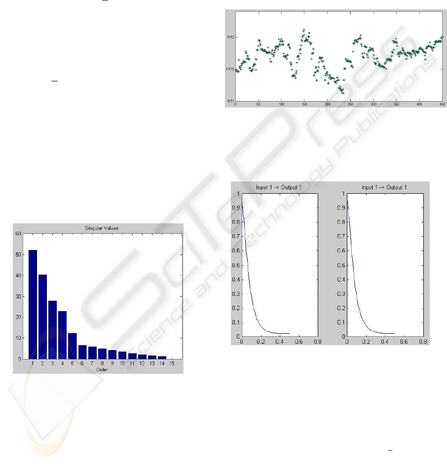
6 NUMERICAL EXAMPLE
It was considered a ”real-life” process (van Overschee
and de Moor, 1996), a laboratory setup acting like
a dryer. The order is four and it can be determined
through the singular values, shown in figure 1.
Figure 1: Singular values of the sytem, for the first 200 mea-
surements. We have assumed that the order of the system is
4.
There is one input only, the voltage over the heat-
ing device (a mesh of resistor wires), and one output,
the air temperature, measured by a thermocouple at
the output – air is fanned through a tube and heat-
eds at the inlet. We have compared only the 1QR
versions, since they produce basically the same es-
timates than the 2QR versions, using i = 15, a forget-
ting factor of 0.995 in the second least squares prob-
lem of the R-MOESP and, for initialization, we have
used the first 200 samples of a set of 1000. Figure 2
shows a snapshot of the estimated eigenvalues of A,
with both algorithms and the offline version of PO-
MOESP (N=200 to N=650). They are all very close
and converging to the true values. In figure 3, we
show the frequency response of the estimated system,
for the offline R-MOESP algorithms (left) and the re-
cursive R-MOESP-1QR algorithm (right), for the first
350 measurements.
Figure 2: Snapshot (N=200 to N=650) of the trajectory
of the estimated eigenvalues, for the algorithms here pro-
posed (version 1QR) and the offline version of PO-MOESP
(N=200 to N=650).
Figure 3: Frequency response of the offline estimated sys-
tem (left) and the recursive estimated system (right).
As to the numerical efficiency, the main differ-
ences between the proposed algorithms lie in the first
step. In fact, when dealing with LQ decompositions,
a small difference in the size of two matrices has a
big effect on the number of flops required to complete
a LQ decomposition: approximately
¡
4
3
n
3
r
+ 2n
2
r
¢
flops (Golub and van Loan, 1996), on a n
r
×(n
r
+ 1)
matrix (the size of matrices in the online algorithms).
If we compare the less efficient algorithm from Van
Overschee and De Moor (n
r
= 2 (m + l) i = 180)
with its most efficient version, the R-MOESP-1QR
(n
r
= (2m + l) i + l = 138), we can see that less
RECURSIVE MOESP TYPE SUBSPACE IDENTIFICATION ALGORITHM
181

than 23% in the number of rows produces less 57.7%
of the number of flops (7.8 · 10
6
in the Van Over-
schee and De Moor’s algorithm and 3.31 · 10
6
in the
R-MOESP-1QR version).
7 CONCLUSIONS
In this paper some algorithms for subspace on-line
identification have been introduced. They are based
on the PO-MOESP (Verhaegen, 1994) and R-MOESP
(van Overschee and de Moor, 1996) techniques, and
therefore implemented through LQ decompositions.
However, unlike the original algorithms, the proposed
recursive algorithms are based on a least squares in-
terpretation of the orthogonal projections. In fact, Z
i
,
Z
i+1
and even Z
i
Π
U
f
⊥
are related to least squares
problems. This allows us to deal with LQ decompo-
sitions of smaller matrices, improving the numerical
efficiency of the algorithms without any loss of accu-
racy. We can also use a modified Householder algo-
rithm, specially developed to improve the efficiency
of this LQ-based least squares problems.
Two versions were proposed: the 2QR, where two
LQ decompositions are needed to compute Z
i
, Z
i+1
and even Z
i
Π
U
f
⊥
, and the 1QR version, where only a
single LQ decomposition is needed. This last version
is, as expected, more efficient (and therefore more in-
teresting) than the first one. However, when compared
with the iterative version developed directly from the
offline algorithm, the 2QR may also be more efficient
than the later. This happens due to the size of the ma-
trices involved. In fact, the LQ decomposition of a
n
r
× (n
r
+ 1) matrix (the size of matrices in the on-
line algorithms), needs approximately
¡
4
3
n
3
r
+ 2n
2
r
¢
flops (Golub and van Loan, 1996). This means that
two LQ decompositions of lower dimension matrices
may be more efficient than one single LQ decomposi-
tion, of a matrix with bigger n
r
.
Further improvements will be made, in order to
consider the update (although partial) of the singu-
lar value decomposition. It is also expected the more
accurate study of the convergence question.
REFERENCES
Chiuso, A. and Picci, G. (2001). Asymptotic variance of
subspace estimates. In Proc. CDC’01 - 40th Con-
ference on Decision and Control, Orlando, Florida,
USA, pages 3910–3915.
Cho, Y., Xu, G., and Kailath, T. (1994). Fast recursive iden-
tification of state space models via exploitation of dis-
placement structure. Automatica, 30:45–59.
Delgado, C. and dos Santos, P. L. (2004a). Analysis and
efficiency improvement of the estimation of matrices
a and c in some subspace identification methods. In
Proc. SICPRO’05 – 4th International Conference on
System Identification and Control Problems, Moscow,
Russia (Accepted for Publication).
Delgado, C. and dos Santos, P. L. (2004b). Exploring the
linear relations in the estimation of matrices b and d in
subspace identification methods. In Proc. ICINCO’04
– 1st International Conference on Informatics in Con-
trol, Automation and Robotics, Set
´
ubal, Portugal.
dos Santos, P. L. and de Carvalho, J. L. M. (2003). Improv-
ing the numerical efficiency of the b and d estimates
produced by the combined deterministic-stochastic
subspace identification algorithms. In Proc. CDC’03
– 42nd Conference on Decision and Control, Maui,
Hawaii, USA, pages 3473–3478.
dos Santos, P. L. and de Carvalho, J. L. M. (2004). A new
insight to the a and c matrices extraction in a MOESP
type subspace identification algorithm. In Proc. Con-
trolo’04 – 6th Portuguese Conference on Automatic
Control, Faro, Portugal.
Golub, G. and van Loan, C. (1996). Matrix Computations.
Johns Hopkins University Press, 3rd edition.
Gustafsson, T., Lovera, M., and Verhaegen, M. (1998).
A novel algorithm for recursive instrumental variable
based subspace identification. In Proc. CDC’98, Con-
ference on Decision and Control, pages 3920–3925.
Larimore, W. (1990). Canonical variate analysis in identifi-
cation, filtering and adaptive control. In Proc. CDC’90
– 29th Conference on Decision and Control, pages
596–604.
Ljung, L. (1983). Theory and Practice of Recursive Identi-
fication. The MIT Press.
Ljung, L. (1987). System Identification: Theory for the
User. Prentice-Hall.
Moonen, M., de Moor, B., Vandenberghe, L., and Vande-
walle, J. (1989). On- and off-line identification of lin-
ear state space models. International Journal of Con-
trol, 49:219–232.
Oku, H. and Kimura, H. (2000). Recursive algorithms of
the state-space subspace system identification. Auto-
matica.
van Overschee, P. and de Moor, B. (1996). Subspace Iden-
tification for linear systems. Kluwer Academic Pub-
lishers.
Verhaegen, M. (1994). Identification of the deterministic
part of MIMO state space models given in innovations
form from input-output data. Automatica, 30:61–74.
Viberg, M., Ottersten, B., Wahlberg, B., and Ljung, L.
(1991). Performance of subspace based state-space
systems identification methods. In Proc. IFAC’91 –
12th IFAC World Congress, Sydney, Australia.
ICINCO 2004 - SIGNAL PROCESSING, SYSTEMS MODELING AND CONTROL
182
