
A VISUAL SERVOING ARCHITECTURE USING PREDICTIVE
CONTROL FOR A PUMA560 ROBOT
Paulo Ferreira
Escola Superior de Tecnologia de Setúbal, Estefanilha, 2914-508
João C. Pinto
Instituto Superior Técnico, Av. Rovisco Pais, 1096 Lisboa, Portugal
Keywords: robotic manipulators, predictive control, vision, modelling, simulation.
Abstract: A control system for a six degrees freedom Puma robot using a Visual Servoing architecture is presented.
Two different predictive controllers, GPC and MPC, are used. A comparison between these two ones and
the classical PI controller is performed. In this system the camera is placed on the robot’s end-effector and
the goal is to control the robot pose to follow a target. A control law based on features extracted from
camera images is used. Simulation results show that the strategy works well and that visual servoing
predictive control is faster than a PI control
.
1 INTRODUCTION
The controller has a crucial role in the visual
servoing system performance. Most of the developed
works in visual servoing systems do not take into
account the dynamics of the manipulator.
The term Model Predictive Control (MPC)
includes a very wide range of control techniques
which make an explicit use of a process model to
obtain the control signal by minimizing an objective
function (
Camacho 98). The MPC is formulated
almost often in a state space form conceived for
multivariable constrained control, Generalized
Predictive Control (GPC), which was first
introduced in 1987 (Clarke et al., 1987), is primarily
suited for single variable and the model is presented
in a polynomial form. Model Predictive control has
been adopted in industry as an effective way of
dealing with multivariable constrained control
problems (Lee and Cooley 1997). A work developed
in the field of visual servoing used a predictive
controller in small displacements (Gangloff, 98).
Other work compares a GPC with respect to a PID
and a feedforward controller in a pan-tilt camera
(Croust, 99).
To carry out this work it was created a toolbox
that allows incorporating vision in the Puma control
architecture. Its great versatility, allowing the easy
interconnection of different types of controllers,
becomes this type of tools very advantageous. The
Puma 560 model and the used 2D visual servoing
architecture can be found in (Ferreira 2003). In this
paper the results of a set of experiences in the area of
the modelling, identification and control of a visual
servoing system for a Puma 560 are presented.
This paper is organised as follows: Section 2
introduces the principles of Predictive Control (GPC
and MPC) and the identification of the Puma
ARMAX model. The experimental settings and the
results for a PI, a GPC and a MPC controller are
given in section 3. Section 4 concludes the paper and
section 5 suggests the continuity of this work.
2 PREDICTIVE CONTROL
2.1 Generalized Predictive Control
The basic idea of GPC is to calculate a sequence of
future control signals in such a way that it minimizes
a cost function defined over a prediction horizon
(E.F.Camacho 1998).
The system model can be presented in the ARMAX
form (Camacho 98):
475
Ferreira P. and C. Pinto J. (2004).
A VISUAL SERVOING ARCHITECTURE USING PREDICTIVE CONTROL FOR A PUMA560 ROBOT.
In Proceedings of the First International Conference on Informatics in Control, Automation and Robotics, pages 475-478
DOI: 10.5220/0001147204750478
Copyright
c
SciTePress

1
1
11
1
)()(
)()()()(
−
−
−−
−
+−=
z
tzC
TtuzBtyzA
e
ξ
(1)
Where A(z
-1
), B(z
-1
) and C(z
-1
) are the matrix
parameters of transfer function H(z). To compute the
output predictions is necessary to know the system
model that must be controlled (Fig. 1).
Figure 1: Manipulator system block diagram controlled by
vision
.
The parameters used by the GPC are obtained
from the configuration shown in figure 7 and the
transfer function is given by:
1
() 11
() ()
*( ) 2 1
a
cc
T
pz z
HZ JFzJ
pz z z
−
+
==
−
&
(2)
The parameters of this function are used in
predictive controller implementation.
The robot model is obtained by identifying each
of the joints dynamics to obtain a six order linear
model:
0
1
1
2
2
3
3
4
4
5
5
6
0
1
1
2
2
3
3
4
4
5
5
)(
azazazazazaZ
bzbzbzbzbzb
ZF
i
++++++
+++++
=
−−−−−−
−−−−−
System Identification .In the identification procedure
is used a PRBS as input signal. A prediction error
method (PEM) was used to identify the Robot
dynamics. The noise model C(z
1
) of order 1 was
selected. In this approach the identification of H(Z)
(Fig.1) is performed around a reference condition.
Since the robot is controlled in velocity and because
the dynamics depend almost from the first joints and
the displacement is small is possible to linearize the
system in turn of the position q. It was also
necessary to consider a diagonal inertia matrix.
Assuming those conditions, is possible to consider
that the Jacobian matrix is constant and therefore
H(Z). This procedure is valid at low velocities. This
means that the cross coupled terms are neglected.
2.2 A MPC Controller
In this approach the model used is in a space state
format. The model of the plant to be controlled is
described by the linear discrete-time difference
equations:
(1) () (),(0)
0
() ()
x
tAxtButxx
yt Cxt
+= + =
=
⎧
⎨
⎩
(3)
Where x(t) is the state, u(t) is the control input and
y(t) is the output.
Figure 2: State space scheme of the manipulator controlled
in velocity
In Fig. 2 is represented the scheme of a
manipulator controlled in velocity. The parameters
values of A
t
, B
t
and C
t
are obtained from the
prediction error method identification algorithm and
eq.3 is computed by the following definitions:
1
ttt
BBJ CCJAA
−
=
==
The algorithm of the predictive control is:
1. At time t predict the output from the system,
)/(
ˆ
tkty
+
, k=N
1
,N
1
+1,…,N
2
. These outputs
will depend on the future control signals,
)/(
ˆ
tjtu
+
, j=0,1,…,N
3
.
2. Choose a criterion based on these variables and
optimise with respect to
3
,...,1,0),/(
ˆ
Njtjtu
=
+
.
3. Apply
)/(
ˆ
)( ttutu
=
.
4. At time t+1 go to 1 and repeat.
3 EXPERIMENTAL PROCEDURE
3.1 System configuration
The implemented Visual Servoing package allows
the simulation of different kind of cameras. In this
particular case, it was chosen a Costar camera placed
in the end-effector and positioned according with o
z
axis. It was created a target of eight coplanar points
that will serve as control reference. The accuracy of
the camera
position control in the world coordinate
system was increased by the use of redundant
features (Hashimoto, 1998). The centre of the target
corresponds to the point with coordinates (0,0) and
J
c
∫
GPC
ZOH
Robot
velocity
control
ˆ
&
&
&
p
J
-1
q
&
∗
q
&
p∆
*p
&
F(Z)
Vision (Z
-1
)
H(Z)
A
t
*p
&
p
&
∫
C
t
J
-1
J
B
t
±
ICINCO 2004 - ROBOTICS AND AUTOMATION
476

the remaining points are placed symmetrically in
relation to this point. The target pose is referenced to
the Robot base frame. In the case of servoing a
trajectory, the target is remained fixed and the
desired point is variable. As the primitive of the
target points is obtained it is possible to estimate the
operational coordinates of the camera position point.
3.2 2D visual servoing with PI control
In 2D Visual Servoing the image characteristics are
used to control the Robot. Images acquired by the
camera are function of the end effector’s position,
since the camera is fixed on the end effector of the
robot. They are compared with the corresponding
desired images. In the present case the image
characteristics are the centroids of the target points.
Fig. 3 represents the model simulation of the
implemented 2D visual servoing configuration. In
this case CT is a PI controller.
Figure 3: Model simulation of 2D visual servoing
3.3 Predictive Visual servoing
implementation.
In this approach our goal is also to control the
relative pose of the Robot in respect to the target.
The model corresponds to Fig.3 but substituting the
controller – in the first case is used a GPC and in
another is used a controller MPC. The target object
is composed of eight coplanar points. From the
projection of these points in the image frame, the
estimated pose of the object in the sensor frame is
computed (Gangloff 99). In both experiments all the
condition and characteristics of the robot are the
same. The goal is control the end effector from the
image error between a current image and desire
image.
3.4 Visual servoing control results
PI Controller .To eliminate the position error was
chosen a PI controller considering points in
operational coordinates:
p
i
= [0.35 –0.15 0.40 π 0 π]
T
p
d
= [0.45 –0.10 0.40 π 0 π]
T
The points p
i
and p
d
correspond to the Robot
position from which the images used to control the
robot are obtained.
In Fig. 4 it can be observed the
translation and rotation of the end-effector around o
x
,
o
y
and o
z
axis.
Figure 4: Stabilization in a desire point using a PI.
Predictive GPC Visual servoing control. In this case
it was used a 2D visual servoing architecture with a
GPC controller. To compare the performance of this
system the same initial and desire position were
used.
Figure 5: Results of a 2D architecture using a GPC
controller.
When compared with the 2D visual servoing
with a PI controller it can be seen that the GPC has a
more linear trajectory and is faster for the same
displacement (more displacement around the x and y
axes). Figure 5 and 6 show that the rise time to PI is
around 0.6s while to the GPC and MPC are 0.1s and
0.2s.The settling time is 1s for the PI, 0.3s for the
GPC and 0.9s for the MPC.
Predictive MPC Visual servoing control. In this case
it was used a MPC controller. To compare the
performance of this system the same initial and
desire position were used.
From Figure 6, it can be seen that the rise time
for the MPC is 0.3s. The result was not so good
ZOH
q
in q
out
Puma 560 +
control
J
r
v
J
+
−
S
CT
pd
d
p
,p
d
dp
P-P*
S
0
A VISUAL SERVOING ARCHITECTURE USING PREDICTIVE CONTROL FOR A PUMA560 ROBOT
477
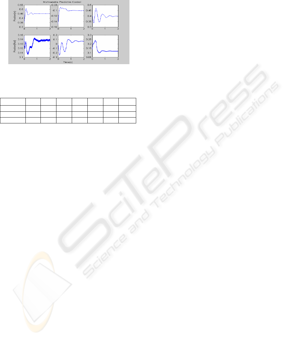
mainly in turn of z and for rotation of the end-
effector.
Figure 6: Results of a 2D architecture using a MPC
controller .
Table 1: r.m.s. values for the control algorithm
SSR
T
x
T
y
T
z
θ
x
θ
y
θ
z
error
PI 2.50 2.40 1.20 2.20 0.30 0.47 1.51
GPC 2.14 0,81 0.22 1.84 0.22 0.02 0.87
MPC 1.36 0.67 3.01 0.76 6.3 6.21 3.04
Table 1 presents the computer errors for each
algorithm which reveals the best performance for the
GPC.
4 CONCLUSIONS
A vision control system for a six degrees of freedom
robot was studied.
A prediction error method was used to identify the
Robot dynamics and implement a predictive control
algorithm ( MPC and GPC).
The controllers (PI, GPC and MPC) were used to
control the robot in a 2D visual servoing
architecture.
The three different algorithms always converge to
the desired position. In general we can conclude that
in visual servoing is obvious the good performance
of both predictive controllers.
The examples show also that the 2D algorithm
associated with the studied controllers allow to
control larger displacements than those referred in
(Gangloff 99).
From the analysis of r.m.s error presented in Table 1
we can conclude the better performance of the GPC.
In spite of better MPC results for the translation in
the xy plane when compared to the GPC, the global
error is worse. These results can still eventually be
improved through a refinement of the controllers
parameters and of the identification procedure. In the
visual servoing trajectory is obvious the good
perfomance of this approach. The identification
procedure has a great influence on the results.
The evaluation of the graphical trajectories and the
computed errors allow finally concluding that the
GPC vision control algorithm leads to the best
performance.
5 FUTURE WORKS
In future works, another kind of controllers such as
intelligent, neural and fuzzy will be used. Other
algorithms to estimate the joints coordinates should
be tested. These algorithms will be applied to the
real robot in visual servoing path planning.
Furthermore others target (no coplanars) and other
visual features should be tested.
ACKNOWLEDGEMENTS
This work is partially supported by the “Programa de
Financiamento Plurianual de Unidades de I&D
(POCTI), do Quadro Comunitário de Apoio III” by
program FEDER and by the FCT project
POCTI/EME/39946/2001.
REFERENCES
Bemporad, A. and M. Morari 1999. Robust Model
Predictive Control: A Survey. Automatic Control
Laboratory, Swiss Federal Institute of
Technology(ETH) Physikstrass
Camacho, E. F. and C. Bordons 1999. Model Predictive
Control. Springer Berlin
Clarke, D.W., C.Mohtafi, and P.S.Tuffs. Generalized
Predictive Control-Part I. The Basic Algorithm,
Automatica, Vol.23, Nº2, pp.137-148
Corke, P. 1996. Visual Control of Robots. Willey
Corke, P. 1994. A Search for Consensus Among Model
Parameters Reported for the Puma 560 In Proc. IEEE
Int. Conf.. Robotics and Automation, pages 1608-1613,
San Diego.
Ferreira, P. e Caldas, P. (2003). 3D and 2D Visual
servoing Architectures for a PUMA 560 Robot, in
Proceedings of the 7
th
IFAC Symposium on Robot
Control, September 1-3, , pp 193-198.
Gangloff, J. 1999. Asservissements visuel rapides D’ un
Robot manipulateur à six degrés de liberté. Thèse de
Doutorat de L’ Université Louis Pasteur.
Lee, J.H,. and B. Cooley-Recent advances in model
predictive control.In:Chemical Process Control,
Vol.93, no. 316. pp201-216b. AIChe Syposium Series
– American Institute of Chemical Engineers.
Mezouar, Y. and F. Chaumette 2001. Images Interpolation
for Image- Based control Under Large Displacements.
Proceedings of the European Control Conference, pp.
2904-2909
.
ICINCO 2004 - ROBOTICS AND AUTOMATION
478
