
REAL-TIME POSITION CONTROL OF A PNEUMATIC SYSTEM
USING MODEL PREDICTIVE CONTROL
Doruk Akyıldız, Umut Karahan, Can Özsoy
Faculty of Mechanical Enginnering, Istanbul Technical University, Gümüssuyu, Istanbul, Turkey
Keywords: Pneumatic System, Model Predictive Control, Dynamic Matrix Control, Real-Time Control
Abstract: Studies on the precise control applications with pneumatic systems have been growing in recent years.In
addition to this, due to the complexity and non-linearity of the system the expected performance will only
be gained by applying modern control strategies. So the subject of this paper is identification and real-time
model predictive control of a pneumatic system. In order to realise system identification, a white noise
signal is sent to the plant and the displacement outputs are stored. Afterwards these data are digitally
processed and the parametric single-input single-output step response model is obtained. In the previous
study on this system with a PD controller, a steady-state error is observed. In order to eradicate this, a
Model Predictive Control – Dynamic Matrix Control algorithm is applied. To run this, in real-time, a
programme is written in Matlab - Simulink and by using the code generated by Matlab - Real-Time
Workshop, the real-time position control of the system is performed.
1 INTRODUCTION
Pneumatics technology is preferred in industry
because it has relatively lightweight and cheap
components. Pneumatic actuators are extensively
used in position control applications with open-loop
control mode where the strokes of the moving parts
are fixed by the mechanical stops. A closed-loop
control system is generally not common due to the
problems arising from air compressibility, poor
damping ability, mechanical frictions, nonlinearities
etc. Because of these regulations studies on the
precise control applications with pneumatic systems
employing advanced control techniques of sliding
mode control, variable structure control, PWM
control, adaptive tracking control etc. instead of
conventional PID have been increased in recent
years. In this paper we present a scheme to use one
of the most popular control strategies, model
predictive control, in order to control the system
precisely.
2 PNEUMATIC SYSTEM
MATHEMATICAL MODEL
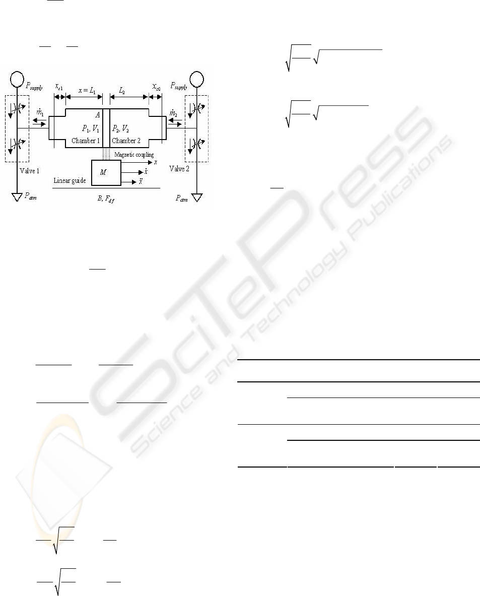
Pneumatics system mathematical model consists of
two parts: The first part is piston dynamics defining
motion of the piston, carriage and payload masses,
the second is thermodynamical pressure dynamics
defining pressure variations in the chambers
according to piston motion and air mass flow rate,
which depends on valve dynamics [1, 2].
2.1 Piston Dynamics
The dynamics of piston motion is described by:
12
()
df
M
xBxF AP P
+
+= −
&& &
(1)
where M is the total moving mass, x is the
position of the piston, B is the viscous-friction
coefficient,
df
is the dry friction forces (static or
dynamic according to piston velocity), A is the
piston cross-sectional area of the rodless cylinder
and
12
are the chamber air pressures, as shown
on Figure 1.
F
,PP
12
()
df
F
MB
xxPP
A
AA
+=−−
&& &
(2)
108
Akyildiz D., Karahan U. and Özsoy C. (2004).
REAL-TIME POSITION CONTROL OF A PNEUMATIC SYSTEM USING MODEL PREDICTIVE CONTROL.
In Proceedings of the First International Conference on Informatics in Control, Automation and Robotics, pages 108-113
DOI: 10.5220/0001147401080113
Copyright
c
SciTePress
Where
df
F
A
is the pressure equivalent of the dry
friction force [7].
net
BA
vvP
M
M
=− + ∆
&
(3)
Figure 1: Schematic diagram of pneumatic system.
Where v and x=
&
12
()
df
net
F
PPP
A
∆=−−
(4)
2.2 Pressure Dynamics
The dynamics of pressures and can be
expressed as [3]:
1
P
2
P
11
11
11
() ()
oo
fP
PS x
x
xxx
=−γ
++
&
&
(5a)
22
22
22
()()
oo
fP
PS
Lx x Lx x
=+γ
+− +−
&
&
x
(5b)
12
LL L=+ (6)
Where S
1
and S
2
are the valve cross-sectional
areas, γ is the ratio of specific heats,
L is the stroke
of the piston (
1
and
2
are shown in Figure 1),
1o
L L
x
and
2o
x
are the position increments for dead
volumes of the chambers,
and are nonlinear
functions of the form
1
f
2
f
1
1
111
11
2
d
u
u
P
TR
fPY
A
TP
⎛⎞
γ
=
⎜⎟
⎝⎠
(7a)
2
2
222
22
2
d
u
u
P
TR
fPY
A
TP
⎛⎞
γ
=
⎜⎟
⎝⎠
(7b)
Here R is the universal gas constant, T
1
and T
2
are the temperatures of the air inside the chambers,
and are assumed to be constant,
ui
and
di
are
upstream and downstream pressures respectively (
i =
1, 2). And,
P P
2/( 1)
() (2/( 1))
1
ii
Yr
γ−
γ
=γ+
γ+
for
00.5
i
r 28
≤
≤ (8a)
2/ ( 1)/
()
1
ii i i
Yr r r
γ
γ+ γ
γ
=−
γ−
for
0.528 1
i
r
<
≤ (8b)
Where
di
i
ui
P
r
P
=
ui
and
di
are assumed to take the values in
Table I according to operation of the valves.
P P
The input signals applied to the valves control
the chamber reference pressures instead of orifice
areas as the valves are of servo operation through
pressure feedback.
()
iiirefi
SkP P
=
−
(9)
(1,2)i =
Where
ir
is the reference pressure for the i-th
chamber and
is the coefficient for i-th valve.
ef
P
i
k
TABLE I
AND VALUES
ui
P
di
P
Valve no
(i)
Valve operation
ui
P
di
P
Connected to supply
sup
p
ly
P
1
0.9
P
1
Open to the atmosphere
1
P
0.9
at
m
P
Connected to supply
sup
p
ly
P
2
0.9
P
2
Open to the atmosphere
2
P
0.9
at
m
P
The relationship between the input voltage and
output reference pressure is described by
iref i i i i oi
Pabuua
=
+>
(10a)
(1,2)i =
0
iref atm i oi
PP ua
=
≤≤
(1
(10b)
,2)i =
Where
i
,
i
and
oi
a
are constant values, is
the input voltage for
i-th valve.
a b
i
u
REAL-TIME POSITION CONTROL OF A PNEUMATIC SYSTEM USING MODEL PREDICTIVE CONTROL
109

3 MODEL PREDICTIVE
CONTROL
Model Predictive Control refers to a class of
algorithms that compute a sequence of manuplated
variable adjustments in order to optimize the future
behaviour of a plant. So the term Model Predictive
Control does not designate a specific control
strategy but a very ample range of control methods
which make an explicit use of a model of the process
to obtain the control signal by minimizing an
objective function. In this study we used one of
these methods named Dynamic Matrix Control (also
called “Cutler’s Method”). The process model
employed in this formulation is the step response of
the plant, while the distrubance is considered to
obtain constant along the horizon. The procedure to
obtain the predictions is as follows:
As a step response model is employed:
y(t) =
1
(i
i
)
g
ut i
∞
=
∆−
∑
(11)
the predicted values along the horizon will be:
ŷ(t + k │ t)=
∑
ň(t + k│ t)=
=
+ +
∞
=
+−+∆
1
)(
i
i iktug
∑
=
−+∆
k
i
i
iktug
1
)(
∑
∞
+=
−+∆
1
)(
ki
i
iktug
+
ň(t + k │ t) (12)
Disturbances are considered to be constant, that
is
ň(t + k │ t) = ň(t │ t) = y
m
(t) – ŷ(t│ t). Then it
can be written that:
ŷ(t + k │ t) = +
+
+y
∑
=
−+∆
k
i
i
iktug
1
)(
∑
∞
+=
−+∆
1
)(
ki
i
iktug
m
(t)– =
∑
∞
=
−∆
1
)(
i
i
itug
=
+ f(t + k) (13)
∑
=
−+∆
k
i
i
iktug
1
)(
where f(t + k) is the free response of the system, that
is, the part of the response that does not depend on
the future control actions and given by:
f(t + k) = y
m
(t) + (14)
)()(
1
itugg
i
iik
−∆−
∑
∞
=
+
As only a finite number of terms (
N) are
considered, the process is assumed to be stable and
casual and therefore the free response is computed
as:
f(t + k) = y
m
(t) + (15)
)()(
1
itugg
N
i
iik
−∆−
∑
=
+
If this equation is expressed in matrix form:
(1)
(2)
()
ft
ft
f
tk
+
⎡
⎤
⎢
⎥
+
⎢
⎥
⎢
⎥
⎢
⎥
+
⎢
⎥
⎣
⎦
M
=
()
()
()
m
m
m
yt
yt
yt
⎡
⎤
⎢
⎥
⎢
⎥
⎢
⎥
⎢
⎥
⎢
⎥
⎣
⎦
M
+
*
*
23 N N112 N-1N
34 N1N21
k1 k2 kN-1 kN
g g g g g g g
g g g g g
g g g g
g +
++
++ + +
⎡⎤
⎢⎥
⎢⎥
−
⎢⎥
⎢⎥
⎢⎥
⎣⎦
LL
L
MMOM M
L
2N-1N
12 N-1N
g g g
g g g g
⎛⎞
⎡⎤
⎜⎟
⎢⎥
⎜⎟
⎢⎥
⎜⎟
⎢⎥
⎜⎟
⎢⎥
⎜⎟
⎢⎥
⎣⎦
⎝⎠
L
MMOM M
L
(1)
(2)
()
ut
ut
ut N
∆−
⎡
⎤
⎢
⎥
∆−
⎢
⎥
⎢
⎥
⎢
⎥
∆−
⎢
⎥
⎣
⎦
M
(16)
The prediction horizon
p for the DMC algorithm
is taken into account. The DMC technique allows
for
m consecutive changes in the input variable (m ≤
N), m being called the control horizon. In this way
the changes in the model output over the prediction
horizon due to consecutive changes in the input
variable over the control horizon, can be expressed
as:
ŷ(t + 1 │ t) = g
1
∆u(t) + f(t + 1)
ŷ(t + 2 │ t) = g
2
∆u(t) + g
1
∆u(t + 1) + f(t + 2)
.
.
.
ŷ(t + p│t)= +f(t + p) (17)
∑
+−=
−+∆
p
mpi
i
iptug
1
)(
Defining the system’s dynamic matrix G as:
G =
1
21
mm-1 1
pp-1
g 0 0
g g 0
g g g
g g
L
L
MMOM
L
MMOM
p
-m 1 g +
⎡
⎤
⎢
⎥
⎢
⎥
⎢
⎥
⎢
⎥
⎢
⎥
⎢
⎥
⎢
⎥
⎢
⎥
⎣
⎦
L
(18)
The prediction can be computed by the general
known expression:
ŷ = Gu + f (19)
ICINCO 2004 - INTELLIGENT CONTROL SYSTEMS AND OPTIMIZATION
110
The objective of a DMC controller is to drive the
output as close to the setpoint as possible in a least
squares sense with the possibility of the inclusion of
a penalty term on the input moves.Therefore, the
manipulated variables are selected to minimize a
quadratic objective that can consider the
minimization of the future errors and the control
effort, in which case it presents the generic form;
J = [ŷ(t + j │ t) – w(t + j)]
∑
=
p
j
1
2
+
∑
λ[∆u(t + j – 1)]
=
m
j 1
2
(20)
If there are no constraints, the solution to the
minimization of the cost function
J = ee
T
+ λuu
T
,
where
e is the vector of future errors along the
prediction horizon and
u is the vector composed of
the future control increments ∆
u(t) , ... , ∆u(t + m),
can be obtained analytically by computing the
derivative of
J and making it equal to 0, which
provides the general result:
u = (G
T
G + λI)
-1
G
T
(w – f) (21)
As in all predictive strategies, only the first
element of vector u is really sent to the plant. It is
not advisable to implement the entire sequence over
the next m intervals.This is because is impossible to
perfectly estimate the disturbance vector and
therefore it is also impossible to anticipate precisely
the unavoidable disturbances that cause the actual
output differ from the predictions that are used to
compute the sequence of control
actions.Furthermore, the setpoint can also change
over the next m intervals.
4 SYSTEM IDENTIFICATION
In section 3, it was mentioned that DMC algorithm
uses a single-input single-output step response
model, to calculate the control signals. In order to
obtain these model coefficients, a system
identification process has been realized by using
Matlab - System Identification Toolbox.
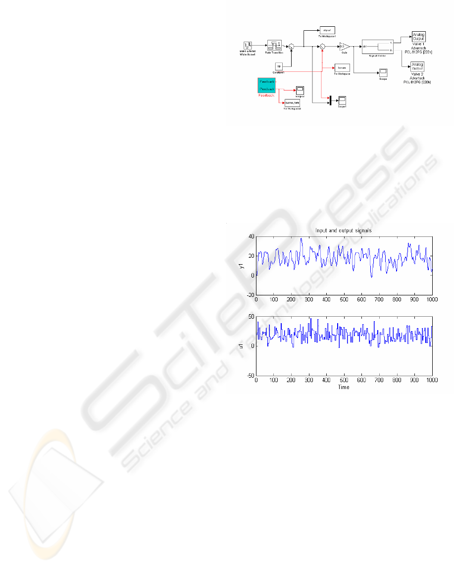
The Simulink model, which was developed for
data acquisition is shown in Figure 2.
Figure 2: The Simulink Model for System
Identification.
The SISO Step response Model is obtained by
sending a white noise signal to the plant. The white
noise signal and the response of the plant is given in
Figure 3.
Figure 3: Input and Output Signals.
In Figure 3, u1 is the white noise signal and y1 is the
osition signal of the plant. p
After the system identification process, the
validation is carried out and the validation results
indicate a 3
rd
order system model. The measured and
computed values are given in Figure 4 and the unit
step response of this 3
rd
model is given in Figure 5.
REAL-TIME POSITION CONTROL OF A PNEUMATIC SYSTEM USING MODEL PREDICTIVE CONTROL
111
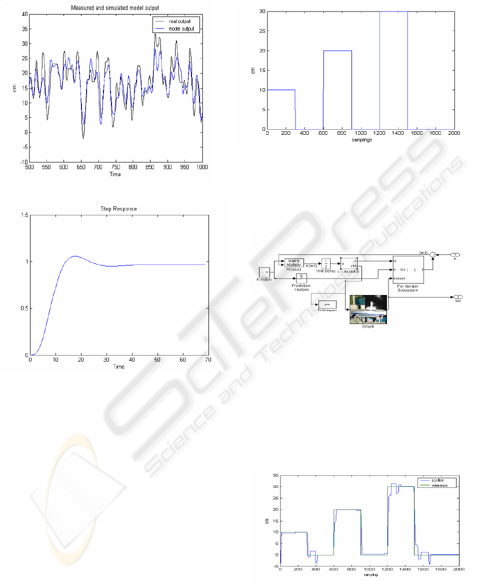
Figure 4: The Validation Results.
Figure 5: Unit Step Response of 3
rd
Order SISO
Model.
5 REAL - TIME POSITION
CONTROL
The feedback gain matrix was built by the step
response coefficients which were calculated offline
and shown in Figure 5. Afterwards the algorithm
applied to the system and twelve real-time position
control trials were realised. The reference trajectory
for these trials is chosen as in Figure 6.
Figure 6: Reference Trajectory.
For real-time control purposes, Matlab - Simulink -
Real-Time Workshop Toolbox is used. A Simulink
model containing the dynamic matrix control
algorithm and signal conditioners are prepared. The
main block is shown in Figure 6.
Figure 6: The Main Simulink Block
In these twelve real-time experiments, controller
parameters, such as prediction horizon and control
horizon, and also the coefficient lambda were
changed. The optimal response is illustrated in
Figure 7. Figure 8 shows the worst among these
experiments.
Figure 7: Optimal Response
(Prediction Horizon: 20, Control Horizon: 20,
Lambda:80)
ICINCO 2004 - INTELLIGENT CONTROL SYSTEMS AND OPTIMIZATION
112

Figure 8: The Worst Response
(Prediction Horizon: 20, Control Horizon: 10,
Lambda:20)
It is observed that in some positions the system
response goes away from the reference and again
starts to follow. This can be explained related to the
high dry friction values in those regions. In the mean
time steady-state errors are eliminated by this
control algorithm as seen in Figure 7.
6 EXPERIMENTAL
INSTALLATION
The system consists of a magnetically coupled
rodless pneumatic cylinder with high precision
guide (SMC CY1HT32, stroke 0.5 m, diameter
0.032 m), two three-way electropneumatic
servovalves (SMC VEP 3121), a magnetic linear
scale (SONY Magnescale SR10-060A, a computer
having a 1.6 GHz microprocessor, 256 MB RAM
and a data acquisition card (Advantech PCL-
812PG). Matlab - Simulink data acquisition software
is used under Windows 98 operating system.
7 CONCLUSION
In this paper we considered a system identification
and a real-time DMC position control on o
pneumatic system. We observed a steady-state error
from the previous studies on the same test bench
with PD controller. In order to eradicate this error
we used Model Predictive Control algorithm.
In Matlab software, it can be seen that there is a
MPC Toolbox which cannot be used in real-time
applications. So we prepared a new real-time usable
Simulink algorithm for unconstrained SISO systems.
The step response coefficients, which are
necessary for the DMC algorithm, were calculated
off-line in this study. It can be said that a self-tuning
DMC application will increase the system’s
performance and will efface the need of an operator.
REFERENCES
Koç, I.M., 1998. Accurate and Robust Pneumatic Position
Control, Master Thesis, Istanbul Technical University,
Institute of Science and Technology, Istanbul.
Cihan, S., 1999. Pneumatic Position Control, Master
Thesis, Istanbul Technical University, Institute of
Science and Technology, Istanbul.
Zorlu, A., 2002. Experimental Modelling and Simulation
of a Pneumatic System, PhD. Thesis, Istanbul
Technical University, Institute of Science and
Technology, Istanbul.
Karahan U., Özsoy C., Kuzucu A., 2003.The real-time
position control of a pneumatic system with rapid
prototyping approach, IFAC Conference, Istanbul.
Camacho E.F., Bordons C., 2000. Model Predictive
Control, Springer-Verlag, London.
Camacho E.F., Bordons C., 1995. Model Predcitive
Control in the Process Industry, Springer-Verlag,
London.
Morari M., 1993. Model predictive control:Multivariable
control technique of choice in the 1990s?, California
Institude of Technology, CIT/CDS 93-024, Technical
Reports.
Qin S.J., Badgwell T.A., 1997. An overview of industrial
model predictive control technology, Chemical
Process Control-AIChE Symposium Series, 232-256
Cutler C. R., Ramaker B. L., 1979. Dynamic matrix
control-a computer control algorithm, AIChE National
Meeting, Houston.
De Keyser R.M.C., Van De Velde G.A., Dumortier
F.A.G., 1988. A comparative study of self-adaptive
long-range predictive control methods, Automatica,
Vol 24, No 2, 149-163.
Pandian, S.R., Hayakawa, Y., Kanazawa, Y., Kamayama,
Y., Kawamura, S., 1997. Practical design of a sliding
mode controller for pneumatic actuators, Transactions
of the ASME, Journal of Dynamic Systems,
Measurement, and Control, 119, 666-674.
Morari M., Ricker N.L., 1998. Matlab Model Predictive
Control Toolbox user’s guide version 1.0, The
Mathworks Inc., Natick.
Ljung, L., 2002. Matlab System Identification Toolbox
user’s guide version 5.0.2, The Mathworks Inc.,
Natick.
Mathworks, 2002. Matlab Real-Time Workshop user’s
guide version 5.0, The Mathworks Inc., Natick.
REAL-TIME POSITION CONTROL OF A PNEUMATIC SYSTEM USING MODEL PREDICTIVE CONTROL
113
