NEW METHOD FOR STRUCTURAL CHANGE DETECTION OF

TIME SERIES AS AN OPTIMAL STOPPING PROBLEM

Hiromichi Kawano, Ken Nishimatsu

NTT Service Integration Laboratories, Musashino-shi, Tokyo, 180-8585 Japan

Tetsuo Hattori

School of Enginieering, Kagawa University, Takamatsu City, Kagawa, 761-0396 Japan

Keywords: Time series, Structural change, Dynamic Programming, Optimal stopping problem

Abstract: In general, an appropriate pred

iction expression and/or model is constructed to fit a time series though, the

model begins to unfit (or not to fit) the time series from some time point, especially in the field that relates

to human activity and social phenomenon. In such case, it will be important not only to quickly detect the

unfitting situation but also to rebuild the prediction model after the detection as soon as possible. In this

paper, we formulate the structural change detection problem in time series as an optimal stopping problem,

using the concept of DP (Dynamic Programming) with a cost function that is the sum of unfitting (or not

fitting) loss and action cost to be taken after detection. And we propose a method for optimal solution and

show the correctness by proving a theorem. Also we clarify the effectiveness by showing the numerical

experimentation.

1 INTRODUCTION

Change point detection (CPD) problem in time series

is to find that a structure of generating data has

changed at some time point by some cause. We

consider that the problem is very important and that

it can be applied to a wide range of application

fields.

For example, degradation detection in

com

munication system (R.Jana and S.Dey, 2000),

object detection on a radar screen ( R.M.Gagliardi

and I.S.Reed, 1965), speech processing (R.J.Di

Francesco, 1990), and fault detection (A.S.Willsky,

1996), (D.Kauame, et al., 1996) are such application

examples of the CPD problem.

The processing method for the CPD problem is

ughly divided into two types: one is batch

processing that checks all generated data in the past

and another is sequential processing that checks if

the structure has changed or not at every new data

generation.

As the former representative method, Chow test

is well kn

own and is often used in econometrics

(Chow,G.C., 1960). It does a statistical test by

setting the hypothesis that the change has occurred at

time t. However, the problem of Chow test exits in

that we have to give the change time t for the

hypothesis setting, and also in that the test lacks the

rapidity to detect the change point.

As the latter representative method, there are

ayes’ method (S.MacDougall, A.K.Nandi and

R.Chapman, 1998), (V.V.Veeravalli and

A.G.Tartakovsky, 2002) and CUSUM one

(E.S.Page, 1954), (C.Han, P.k.Willet and

D.A.Abraham, 1999), (S.D.Blostein, 1991), (Y.Liu

and S.D.Blostein, 1994), (M.Basseville and

I.V.Nikiforov, 1993), (M.Basseville, 1988), based on

sequential probability ratio test. The Bayes’ method

can detect the change point, based on the sequential

estimation of posterior probability, if the generation

distribution of time series data is known at the time

before and after the change point. So the Bayes’

method can solve the problem in the Chow test, but

it requires that the generation distribution for the

time series data is already known.

Kawano H., Nishimatsu K. and Hattori T. (2004).

NEW METHOD FOR STRUCTURAL CHANGE DETECTION OF TIME SERIES AS AN OPTIMAL STOPPING PROBLEM.

In Proceedings of the First International Conference on Informatics in Control, Automation and Robotics, pages 24-31

DOI: 10.5220/0001147500240031

 SciTePress

Moreover, in practical situation, we have to

consider not only that a loss cost is involved with

prediction error but also that an action to be taken

after the change detection will need a cost.

Conversely, the CPD is necessary in order to judge

when to take the action.

Taking the field of network management for

example, time series data (e.g. error rate and delay)

of the quality are always monitored, and when the

structural change is detected, some action for the

quality improvement is taken.

In the structural change detection under such

situations, we must consider the trade-off between

loss by the degradation and cost for the quality

reformation.

However, as far as the authors can know, no

such conventional CPD method considering the

action cost has been proposed, in spite of the fact

that such method is very useful at practical level.

In this paper, in order to solve difficulties in

conventional methods for structural change detection

in time series, we propose a new and practical

method based on an evaluation function of loss cost.

And we formulate the CPD problem as an optimal

stopping problem using the concept of DP (Dynamic

Programming) and give the optimum solution in the

formulation. We consider that our method is

effective in the sense as follows.

1. Differently from the Chow test, it does not need to

set the change point in a priori.

2. Unlike the Bayes’ method, it does not need to give

the generation distribution of time series data.

3. It can quickly detect the structural change point by

the sequential processing.

4. It minimizes the evaluation function that sums up

the loss involved with prediction error and action

cost to be taken after the change detection.

5. It is a meta-level method so that we can apply it to

any prediction model in the evaluation function.

Also in this paper, we present the correctness of our

solution by proving a theorem and show the

effectiveness by numerical experimentation results.

2 FORMULATION

2.1 Evaluation Function

We formulate the CPD problem as an optimal

stopping one based on an evaluation function that

sums up the cost involved by prediction error and

action cost to be taken after the change detection.

For example, a prediction expression is given in the

following equation as a function of time t, where y

, β0, ε mean the function value, two constant

coefficients, and error term, respectively.

⋅

(1)

The error term ε is given as a random variable of the

normal distribution of variance σ and average of 0,

i.e., ε～N(0, σ).

A time series data based on the Equation (1) is

shown in Figure 1, that is generated by making

normal random numbers of average 0 and variance 1

for ε, and by setting β

=0.2, β0=1 for the time

t=1,2,…,70, and β

=0.8, β0=－41 for the time after

t=71.

The tolerant error interval or tolerance zone between

two broken lines as shown in Figure 1 is decided

using the first time series data from t=1 to t=20.

Using those data, the prediction expression is

made by the least squares method, and the tolerant

interval of error is calculated as 95% confidence

interval of the sample variance of residual ε.

Note that the tolerant error interval is not based

on the confidence interval of regression formula

given in the following Equation (2), but is defined

based on the distribution of error term ε of Equation

(1)(

N.R.Draper, H.Smith, 1996).

ˆˆ

β+β=

⎟

⎠

⎞

⎜

⎝

⎛

−

++α−±

)(1

1),2(

(2)

where t, α ,

x , and n denote t distribution,

significance level, average, and the number of data,

respectively, and let

be prediction error in time

, and are defined as follows.

neV

∑

)(

∑

−=

ixx

xxS

1 112131415161718191

obser vat ion

dat a

forecasting

dat a

‐2σ

2σ

Figure 1: Example of time series data.

NEW METHOD FOR STRUCTURAL CHANGE DETECTION OF TIME SERIES AS AN OPTIMAL STOPPING

PROBLEM

In Figure 1, it can be read that the generated

data runs out frequently from the tolerance zone

since after t=70. From the fact, when the difference

(or observation error) between the observed data and

forecasted value exceeds a specified tolerance (i.e.,

when the observed data goes out from the tolerance

zone), we can think that that there is a high

possibility that the structural change has occurred.

For simplicity, we think two situations; one is

the situation that the observed data is out from the

tolerance zone, and another the situation that the

observed data is in the zone. Then we call the former

situation “

unfitting” and the latter “fitting”. Based on

this discussion, we consider that the structure has

changed, when the unfitting occurs between

sequentially observed data and forecasted value by

continuing

N times. This specified tolerance is

defined as, e.g., 2σ of the distribution on error ε that

is estimated at the time when the prediction

expression is made.

The evaluation function is given in (3) as the

sum of two kinds of cost: the damage caused by the

unfitting (i.e., unfitting loss) and action cost to be

taken after the change detection.

Total_cost=cost (

A)+cost(n) (3)

where cost(

n) is the sum of the loss by continuing n

times unfitting before the structural change

detection, and cost(

A) is the cost involved by the

action after the change detection.

Taking the quality control problem for example,

the above cost(

n) means the loss caused by the

quality degradation and superfluous quality. And the

cost(

A) means the cost involved by some facility

replacement.

Since the observed time series data is a random

variable and the unfitting event is stochastic, the

value of the evaluation function Total_cost also

becomes a random variable. Then we have to find

the number of times

N that minimizes the

expectation value of Total_cost, under the

assumption that the structural change occurs

randomly. Note that the evaluation function can be

defined if only the distribution of error ε is given, so

there is no need for the prediction expression to be

such a form like equation (1).

2.2 Structural Change Model

We assume that the structural change is Poisson

occurrence of averageλ , and that, once the change

has occurred during the observing period, the

structure does not go back to the previous one. The

reason why we set such a model is that we focus on

the detection of the first structural change in the

sequential processing (or sequential test). The

concept of the structural change model is shown in

Figure 2.

Figure 2: Structural change model

Moreover, we introduce a more detailed model.

Let

R be the probability of the unfitting when the

structure is unchanged. Let

Rc be the probability of

the unfitting when the structure change occurred. We

can consider that

Rc is greater than R, i.e., Rc>R.

The detailed internal model for the State Ec and

E are illustrated as similar probabilistic finite state

automatons in Figure 3 and 4, respectively.

Figure 3: Internal model of the State E.

Figure 4: Internal model of the State E

out

out in

1-λ

1.0

Ec : State that the structural change occurred.

E : State that the structure is unchanged.

λ : Probability of the structural change

occurrence. (Poisson Process.)

ICINCO 2004 - SIGNAL PROCESSING, SYSTEMS MODELING AND CONTROL

2.3 Evaluation Function Using DP

Let the cost(n) be a・n as a linear function for n,

where

a is the loss caused by the unfitting in one

time. And for simplicity, let

C and A denote the

Total_cost and cost(

A), respectively. Then, the

evaluation function in (3) is denoted as the following

equation (4).

naAC ⋅+=

(4)

Using the concept of the DP (Dynamic

Programming), we introduce a function

obtain the optimum number of times

n that

minimizes the expectation value of the evaluation

function of Equation (4).

),( NnEC

Let

N be the optimum number. Let the function

be the expectation value of the evaluation

function at the time when the unfitting has occurred

),( NnEC

in continuing

n times, where n is less than or equal to

N, i.e., 0≦ n≦ N. Then the function is

recursively defined as in the following equation.

),( NnEC

(if

n=N )

NaANNEC ・

=),(

(5)

(if

n<N )

naSSPNnEC

・・)|(),(

),1())|(1(

NnECSSP

+−+

(6)

where

is the state of unfitting in continuing n

times,

1+n

is the state of fitting for the (n+1)-th

time observed data, and

)|(

1 nn

SSP

is the

conditional probability that the state

1+n

occurs

after the state

The first term in the right-hand side (RHS) of

Equation (6) indicates the expectation value of the

evaluation function at the time when the fitting

happens for the (

n+1)-th time observed data after the

unfitting occurred for continuing

n times.

occurred.

The second term in the RHS of Equation (6)

indicates the expectation value of the evaluation

function at the time when the unfitting happens for

the (

n+1)-th time observed data after the unfitting

occurred for continuing

n times.

Note that, from the definition of the function

, the N that minimizes EC(0,N) is the same

n that minimizes the expectation value of the

evaluation function of (4).

),( NnEC

2.4 Minimization

For the aforementioned EC(0,N), the following

theorem holds, and gives the

n that minimizes the

expectation value of the evaluation function of (4).

Theorem.

The N that minimizes EC(0,N) is given as the largest

number

n that satisfies the following Inequality (7).

)|()(

1−

SSPaAa ・

(7)

where the number

N+1 can also be the optimum one

that minimizes

EC(0,N), i.e., EC(0,N) = EC(0,N+1)

, only if

)|()(

1 NN

SSPaAa

+= ・

Proof (Outline).

Since the strict detailed proof needs many pages, we

present the outline of the proof for the Theorem.

In order to prove this Theorem, we derive a

contradiction with two assumptions under a premise

as follows.

Premise: a number

′

is the largest number n

that satisfies the Inequality (7).

Assumption 1: There exists a number

′

such that

'" NN

and

)',0()",0( NECNEC <

Assumption 2: There exists a number

′

such that

"' NN

and

),0(),0( NECNEC

′

We can derive the above contradiction by three

steps, as described below. At Step 1, we prove the

following fundamental lemmas: Lemma 1-1 and

Lemma 1-2. At Step 2, two lemmas, Lemma 2-1,

and Lemma 2-2, are proved.

Using those lemmas, we can show that the

above Assumption 1 contradicts the Premise.

Similarly, at Step 3, it is proved that the Assumption

2 contradicts the Premise, using two lemmas:

Lemma 3-1 and Lemma 3-2.

(A) Lemmas in Step1

Lemma 1-1:

Let

be the event that the structural change

occurs once during the period of observation in

continuing

n times. Let be the

conditional probability that the

occurs under

the condition that failing occurs in continuing

times. Then,

is an increase function

for

)|(

ncn

SEP

)|(

ncn

SEP

Lemma 1-2:

The conditional probability

)|(

1 nn

SSP

is a

decrease function for

Those Lemmas are strictly proved subsequently

in the Appendix.

(B) Lemmas in Step2

Lemma 2-1:

'" NN

, then

),(),( NNECNNEC

′′′′

′

NEW METHOD FOR STRUCTURAL CHANGE DETECTION OF TIME SERIES AS AN OPTIMAL STOPPING

PROBLEM

Lemma 2-2:

, then, for m ( ),

'" NN <

′′

≤<0

),(),( NmNECNmNEC

′

−

′′

′

−

′′

By putting

′

in the Lemma 2-2, we

have

in case of

),0(),0( NECNEC

′′

′

'" NN

This inequality contradicts the Assumption 1: There

exists a number

such that and

"N '" NN <

)',0()",0( NECNEC <

Lemma 3-1:

, then

"' NN < )','()",'( NNECNNEC ≥

where the equality holds only if

and

1'" += NN

)|()(

'1' NN

SSPaAa

+= ・

Lemma 3-2:

, then, for ( ),

"' NN <

'0 Nm ≤<

),(),( NmNECNmNEC

′

−

′

≥

′′

−

′

where the equality holds only if

and

1'" += NN

)|()(

'1' NN

SSPaAa

+= ・

By putting

in the Lemma 3-2, we have

in case of

'Nm =

)',0()",0( NECNEC ≥

′

This contradicts the Assumption 2: There exists a

number

such that

′′

"' NN

and

),0(),0( NECNEC

′′

′

After all,

),0(),0( NECNEC

′′

≤

′

(

'" NN

), where the equality holds only if

and

′′

′

1'" += NN

)|()(

'' NN

SSPaAa

+= ・

It means that

minimizes . And, when

′

),0( NEC

)|()(

'1' NN

SSPaAa

+= ・

, also minimizes

, i.e.,

1'+N

),0( NEC

)1',0(),0( +

′

NECNEC

This completes the proof of the aforementioned

Theorem.

3 EXPERIMENTATION

3.1 Feature of Evaluation Function

We have experimented the proposed method, and

evaluated the feature of the evaluation function,

using the probability of the structural change

occurrence λ and each constant of the Equation (4),

i.e.

A and a, as parameters.

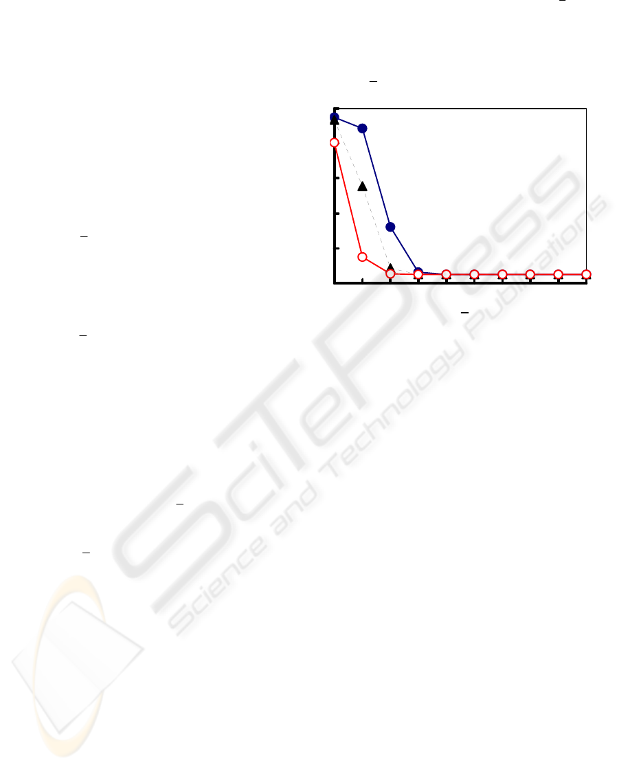
First, by numerical computing, we show the

decreasing situation of the probability

)|(

1−nn

SSP

for

n in Figure 5. In this case, the probability

approaches to 0.05 (5 %) by letting

n become

greater. It meets to the aforementioned Lemma 1-2.

0.2

0.4

0.6

0.8

12345678910

●：

＝0．0001

▲：

＝0．001

○：

＝0．01

)|(

1−nn

SSP

Figure 5: The probability

)|(

1−nn

SSP

for three kinds of

λ (occurrence probability of structural change) in the case

Rc=0.95

That is, we have examined the relation between

the ratio of

aAa /)(

and the optimum number of

times n (that is the same as aforementioned

N), by

varying the probability λ .

Experimental condition:

(i) Structural change probability λ：(three types)

0.1, 0.05, and 0.01.

(ii)

aAa /)(

：1.5～10.0.

(iii)Tolerance of prediction: 2σ of the distribution on

error ε.

(iv)Unfitting probability when the structure is

unchanged:

R=0.1.

(v)Unfitting probability when the structure has

changed:

Rc=0.9.

Result:

The result is shown in Figure 6, where horizontal

axis is

aAa /)(

and vertical axis is n. We can see

that the tendency meets our intuition, as follows.

(i) The optimum number of times

n tends to be

larger when the action cost A after the CPD is

bigger than the unfitting cost

. That is, the n

grows in the case of A > a, because the action

cost A after the change detection becomes

dominant over the loss cost

by prediction

error, and the

n decreases in the case of A < a

for the reverse reason.

ICINCO 2004 - SIGNAL PROCESSING, SYSTEMS MODELING AND CONTROL

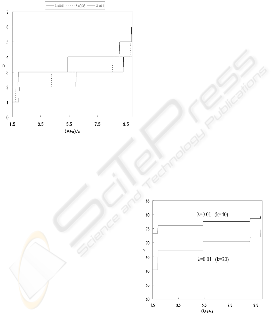
(ii) The n for the CPD increases when the

probability λ of the structural change occurrence

becomes smaller.

Figure 6: Relation between the ratio and the

optimum number of times

aAa /)( +

3.2 Application to Time Series Data

Since the tolerant error in the proposed method is

decided based on the residual sample distribution

when the prediction expression is estimated, the

accuracy of CPD depends on the accuracy of

prediction (or the prediction model). We examine the

fact using the time series data shown in Figure 1.

Outline of experimentation:

(i)Generate the time series data (Figure 1) based on

the Equation (1) as aforementioned in the Section

2.1, by making normal random numbers of

average 0 and variance 1.0 for ε, and by setting

=0.2, β0=1 for the time t=1,2,…,70, and β

=0.8,

β0=－41 for the time after t=71.

(ii)Make prediction expression, using a sequence of

data at the time t=1,…,k from the above generated

time series.

(iii)Decide the tolerant error interval.

(iv)Based on the proposed method, measure the

number of times when the observed data goes out

from the tolerance zone (or tolerant error interval)

for observation data after the time at k+1, and

detect the structural change point.

(v)Perform the above things repeatedly by M times,

and calculate the average of the structural change

point.

Experimental condition:

(i)Tolerant error interval: ± 2σ of the distribution on

error ε.

(ii)The number of data for the decision of prediction

expression: k=20, 40 (2 types).

(iii)Parameter value of the evaluation function:

λ =0.01, and

aAa /)(

is changed in a range of

1.5～10.0.

(iv)Repeating times: M=100.

Result:

The result is illustrated in Figure 7, where horizontal

axis shows

aAa /)(

and vertical axis shows the

detected change point n that is the average of 100

times computation.

Although the detection of the change point depends

on the value of

aAa /)(

, it is expected that the

change point will be detected around the time at

t=70, because the structure of the time series is

changed at t=70. We have verified that the result

meets our intuition very well as follows.

(A) In case of k=20, because the number of the data

for the prediction expression is less than the

case of k=40, the prediction accuracy is

considered to be so much worse. Therefore, the

unfitting frequency increases and the change

point tends to be detected early.

(B) In case of k=40, the change is detected within

the time at t=70～80. We consider that the

proposed method has appropriately detected the

change point.

Figure 7: Detected change point n for the time series in

Figure 1

NEW METHOD FOR STRUCTURAL CHANGE DETECTION OF TIME SERIES AS AN OPTIMAL STOPPING

PROBLEM

4 CONCLUSION

We have proposed a sequential processing method

for structural change detection of time series data,

which we formulated as an optimal stopping

problem with a cost evaluation function. We have

presented the algorithm for the optimum solution,

and have shown the correctness by proving a

theorem. The proposed method is effective in the

sense as follows.

1. Differently from the Chow test, it does not need to

set the change point in a priori.

2. Unlike the Bays’ method, it does not need to give

the generation distribution of time series data.

3. It can quickly detect the structural change point by

the sequential processing.

4. It minimizes the evaluation function that sums up

the loss involved with prediction error and action

cost to be taken after the change detection.

5. It can be applied to any prediction model.

Moreover, we have shown some numerical

experimentation results, where the resultant

situations by obtaining optimum solutions well meet

our intuition and the change point of artificially

generated time series data.

APPENDIX: PROOF OF LEMMA IN

THE STEP 1

Lemma 1-1.

The conditional probability

is an

increase function for

)|(

ncn

SEP

Proof. Based on the model (see Figure 2-4), the

event

is given in (8).

(

)

−

∩=

EEE

(8)

where

E is the event that there is no structural

change,

is the event that the structural change

occurred, and

is defined as .

The probability of the event

defined in (8) is

given as follows.

(

)

(

)

EEPEEPEP

−

∩=

⎟

⎠

⎞

⎜

⎝

⎛

∩=

∑

)(

λλ−=

∑

−

)1(

(9)

Then the joint event between

and , and

the probability are given by (10) and (11),

respectively.

(

⎟

⎠

⎞

⎜

⎝

⎛

∩∩=∩

−

ncnn

EESES

)

(10)

()

cnn

RRESP

−

λλ−=∩

∑

)1(

(11)

Therefore, using (9) and (11), we have

)(

)|(

cnn

ESP

∩

∑

−

λλ−

)1(

(12)

According to the Bayes’ theorem, the posterior

probability

is given by the following

(13).

)|(

ncn

SEP

)()(

)(

)|(

ncnn

cnn

ncn

ESPESP

ESP

SEP

∩+∩

∩

∑

−

λ−+λλ−

λλ−

)1()1(

)1(

nnin

RRR

∑

−

λλ)1(

λ)1(

)(1

nD+

(13)

where

∑

−

λλ)1(

λ)1(

)(

The D(n) is also expressed as the following (14).

ICINCO 2004 - SIGNAL PROCESSING, SYSTEMS MODELING AND CONTROL

∑

−

⎟

⎠

⎞

⎜

⎝

⎛

λ−λ

⎟

⎠

⎞

⎜

⎝

⎛

λ−

)1(

)(

⎟

⎠

⎞

⎜

⎝

⎛

⋅⋅⋅++λ

−

＋

(14)

where

)(1X λ－=

Since

, , and ,

then 0 < X < 1. So, the D(n) becomes a monotonous

decrease for n. Therefore, the probability

of (13) is a monotonous increase

function for n. Lemma 1-1 is proved.

10 <λ≤ 110 ≤λ−<

)|(

ncn

SEP

Remark: Lemma 1-1 indicates that, if the

number of times of the unfitting n increases, the

probability that the structural change has occurred

increases. This meets our intuition clearly.

Lemma 1-2.

The conditional probability

)|(

1 nn

SSP

is a

decrease function for n.

Proof. Based on the model in Fig. 3, we have

))|(1)(1()|(

1 ncnnn

SEPRSSP −−=

)|()1(

ncnc

SEPR−+

(15)

The first term in the RHS of (15) shows the

probability that the fitting occurs for the (n+1)-th

time observed data when the structure is unchanged.

The second term shows the probability that the

fitting occurs for the (n+1)-th time observed data

when the structure changed.

From (15), we have

))(|(1)|(

1 cncnnn

RRSEPRSSP −+−=

(16)

By Lemma 1-2,

is an increase

function, and

, therefore,

)|(

ncn

SEP

RR <

)|(

1 nn

SSP

is a

decrease function for n. Lemma 1-2 is proved.

Remark: Lemma 1-2 indicates that, if the

number of times of continuous unfitting increases,

the probability of the fitting for the next observed

data after those continuous unfitting decreases. This

is intuitively clear, because, by Lemma 1-1, the

probability of the structural change increases if the

number of times of the continuous unfitting

increases.

REFERENCES

R.Jana and S.Dey, 2000. Change detection in Teletraffic

Models. IEEE Trans. Signal Processing, vol.48, No.3,

pp.846-853, March 2000.

R.M.Gagliardi and I.S.Reed, 1965. On the Sequential

detection of Emerging Targets. IEEE Trans.

Information Theory, vol.6, pp.260-263, April 1965.

R.J.Di Francesco, 1990. Real-Time Speech segmentation

Using Pitch and Convexity Jump Models. IEEE Trans.

Acoustics, Speech, Signal Processing, vol.38, pp.741-

748, May 1990.

A.S.Willsky, 1996. A survey of design methods for failure

detection in dynamic systems. Automatica, Vol.12. pp.

601-611, Sept. 1996.

D.Kauame and J.P.remenieras et al., 1996. Effect of The

Compensation In Abrupt Model Change Detection

Problem.

Proc. of IEEE Digital Signal Processing

Workshop, pp.311-314, Sept. 1996.

Chow,G.C., 1960. Tests of Equality Between Sets of

Coefficients in Two Linear Regressions.

Econometrica, Vol.28, No.3, pp.591-605, July 1960.

S.MacDougall, A.K.Nandi and R.Chapman, 1998.

Multisolution and hybrid Bayesian algorithms for

automatic detection of change points.

Proc. of IEEE

Visual Image Signal Processing, vol.145, No.4,

pp.280-286, August 1998.

V.V.Veeravalli and A.G.Tartakovsky, 2002. Asymptotics

of quickest change detection procedures under a

Bayesian criterion.

ITW2002, pp.100-103, Bangalore,

India, Oct. 2002.

E.S.Page, 1954. Continuous inspection schemes.

Biometrika, Vol. 41, pp.100-115, 1954.

C.Han,P.k.Willet and D.A.Abraham, 1999. Some methods

to evaluate the performance of Page's test as used to

detect transient signals. IEEE Trans. Signal

processing, vol.47, No.8, pp.2112-2127, August 1999.

S.D.Blostein, 1991. Quickest detection of a time-varying

change in distribution. IEEE Trans. Information

Theory, vol.37, No.4, pp.1116-1122, July 1991．

Y.Liu, S.D.Blostein, 1994. Quickest detection of an abrupt

change in a random sequence with finite change-time.

IEEE Trans. Information Theory, vol.40, No.6,

pp.1985-1993, Nov. 1994.

M.Basseville and I.V.Nikiforov, 1993. Detection and

Application, Prentice Hall, Inc., April 1993.

M.Basseville, 1988.Detecting Changes in signals and

systems– A survey. Automatica,Vol.24, pp.309-

326, 1988.

N.R.Draper, H.Smith, 1996. Applied Regression Analysis,

John Wiley & Sons Inc, 1966.

NEW METHOD FOR STRUCTURAL CHANGE DETECTION OF TIME SERIES AS AN OPTIMAL STOPPING

PROBLEM