INTELLIGENT ELECTRIC DRIVE SYSTEM
A mechatronics approach
Guy Reginald Dunlop
Department of Mechanical Engineering, Universityof Canterbury, PB4800, Christchurch, New Zealand
Keywords: Mechatronics, Robotics, Intelligent drives, Model based control
Abstract: Drive efficiency is an important consideration in most robotic applications. A hybrid controller for
permanent magnet DC motors has been developed to control the current, and hence the output torque of the
motor. An H bridge is used to provide the basic PWM voltage to the motor, and the controller switches the
bridge between bipolar and unipolar modes in order to minimise the switching losses within the bridge and
motor, and also to minimise the electromagnetic interference. The first application presented is for a
walking robot, and the second is for a dexterous robotic hand. In both cases, control is obtained from a
voltage sourced inverter by means of a tight control loop that uses position readings to infer velocity so that
a full DC motor model can be utilised in the control computer. For the dexterous hand, current control is by
model prediction to avoid the need for direct measurement. The controller and communications are
contained within a small programmable system on a chip which together with a dual H bridge driver is
integrated into small circuit board that is used for distributed control within the hand.
1 INTRODUCTION
Most robots being manufactured are using
permanent magnet electric drives, either DC or
brushless DC. The ideas presented in this paper
apply to both types of drive but discussion will be
restricted to the brushed DC motor.
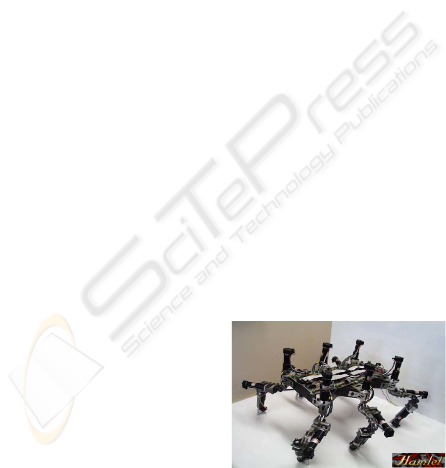
Figure 1: The walking robot Hamlet.
The walking machine Hamlet (Fielding and
Dunlop, 2002) shown in fig. 1 utilises 18 electric
motors. It has 6 legs each of which is operated by 3
DC motors. These can be clearly seen in the
photograph. Each motor contains an integral shaft
position encoder that provides position information
for the kinematic calculations. The position
information from a motor is also used to derive the
velocity of the motor for use in the velocity servo
loop contained inside the position feedback servo
control loop. Hamlet was designed to explore the
omnidirectional walking gaits of insects (Fielding
and Dunlop, 2004) and as such it moves so slowly
that regenerative energy issues need not be
considered. The walker used 6 FPGA (field
programmable array) units to control the 6 legs. The
controllers communicated with off board DSPs via a
single high speed serial bus and the control and
kinematic decisions were computed on the DSPs.
The H bridges were driven in bipolar mode (see
section 2) and were robust enough to withstand brief
current surges during speed reversals or changes.
41
Dunlop G. (2004).
INTELLIGENT ELECTRIC DRIVE SYSTEM - A mechatronics approach.
In Proceedings of the First International Conference on Informatics in Control, Automation and Robotics, pages 41-48
DOI: 10.5220/0001147900410048
Copyright
c
SciTePress
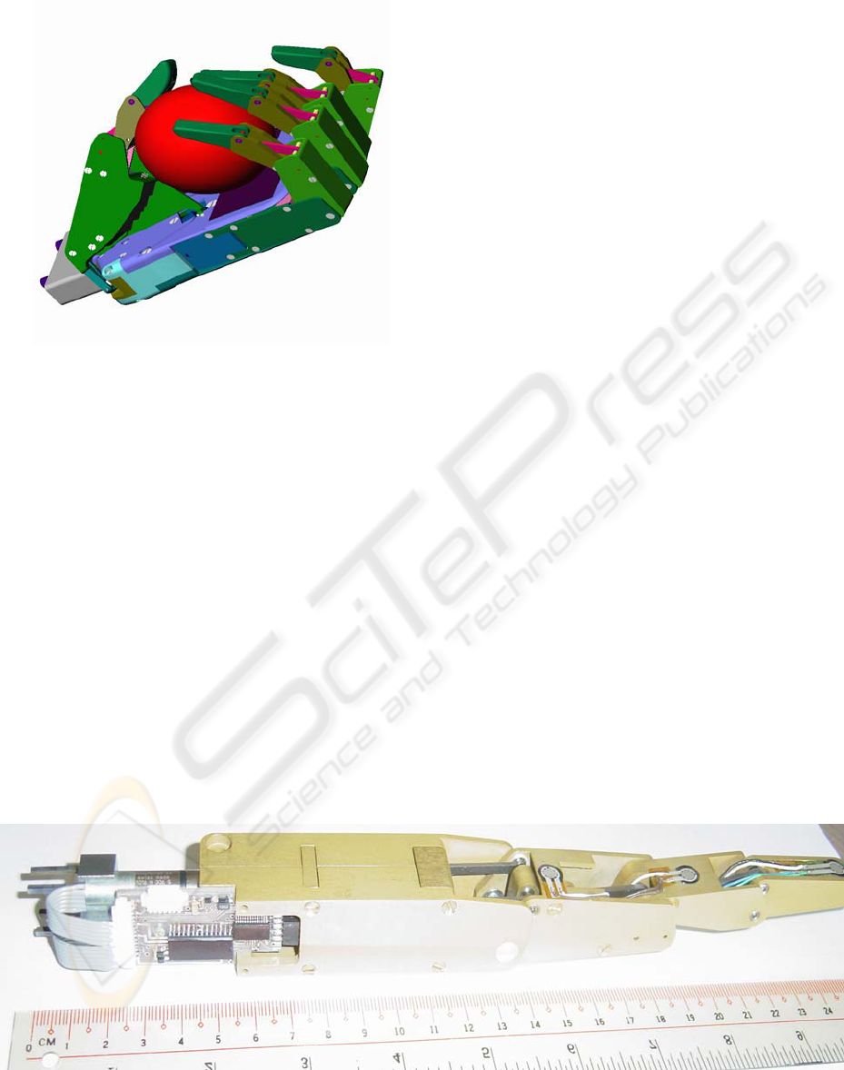
Figure 2: The dexterous Canterbury hand.
The miniature motors within the dexterous hand
shown in fig. 2 are difficult to control as they have
low inertia ironless rotors that have a low “thermal
mass” and are easily overheated. A thermal model
was needed to prevent this, and crucial to its
operation, was precise control of the current in the
motor to reduce resistive heating.
There are a total of 11 DC motors in the hand
and 7 computers so temperature control is of some
importance. As shown in fig.3, each finger contains
2 DC motors with a computer and driver unit. The
heating of the motor armature during the current
pulse needed to break joint stiction is transient, but
the resulting temperature step is superimposed on
top of the temperature within the hand. The need to
minimise the temperature within the enclosed hand
palm space lead to the development a very efficient
drive system using a hybrid switching scheme for
the DC motors. The various motor driving schemes
are discussed in the next section followed by the
application of models for current control which are
presented along with simulation results.
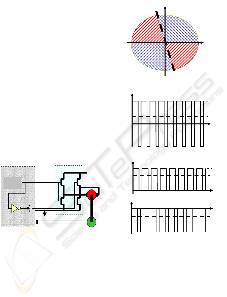
2 BASIC DRIVE STRUCTURE
The purpose of any rotary actuator used in robotics
is to produce torque and speed in a well controlled
manner. This requires four quadrant control of the
torque-speed characteristics of the driver and motor
combination as shown in fig.5(a). No matter which
kind of drive is used, none can handle situation
where the load can drive the motor at a speed where
the back emf is greater than the supply voltage
unless additional overvoltage circuitry is added,
something not required here.
Some commercial constant current IC drivers
provide only two quadrant motor control and can be
destroyed during regenerative operation when
kinetic energy from the motor and robot is absorbed
by the drive. The usual way to avoid this problem is
to use a bipolar drive system that switches at
ultrasonic frequencies so that four quadrant control
is always achieved. However, the cost is more heat
than for a unipolar drive system.
The H bridge driver shown in fig. 4 (4 FETs or
field effect transistors form the left and right
uprights and the motor the cross bar) requires only a
single voltage supply. This is the most commonly
used type of DC motor driver as it uses switching
which is much more efficient than analog amplifier
control. In operation, if FET 1 is on, then FET 3 is
off, and vice versa. Similarly for FETs 2 and 4. The
difference between unipolar and bipolar drive
schemes has been discussed in detail by Tal, and
Persson (1978) so only a brief outline is given here.
Figure 3: A finger from the hand showing the 2 DC motors and the control computer and driver PCB.
ICINCO 2004 - INTELLIGENT CONTROL SYSTEMS AND OPTIMIZATION
42
t
V
18
-18
6
(b) Bipolar PWM
t
V
18
-18
6
(b) Bipolar PWM
t
V
18
0
12
(c) Unipolar PWM +ve
t
V
18
0
12
(c) Unipolar PWM +ve
ω
τ
Bipolar
Unipolar
Unipolar
(a)
τ
= - (k
2
/R)
ω
Bipolar
ω
τ
Bipolar
Unipolar
Unipolar
(a)
τ
= - (k
2
/R)
ω
Bipolar
t
V
-
6
-
18
0
(d) Unipolar PWM -ve
t
V
-
6
-
18
0
(d) Unipolar PWM -ve
Figure 5: Four quadrant torque-speed plot. Motoring is
in quadrants 1 and 3 of (a), and regenerative braking in
quadrants 2 and 4. Efficient operation is obtained by using
the unipolar PWM mode and switching to bipolar mode
for the cross hatched regions in quadrants 2 and 4.
2.1 Bipolar Drives
When operated as a bipolar drive, both sides of the
H bridge are switched on and off in antiphase with
each other so that each end of the motor is connected
alternately between zero volts and the supply
voltage. The FETs act as switches for the current
through the DC motor. FETs 1 and 2 are switched on
for a time
τ
s every T s, and then FETs 3 and 4 are
on for the remaining (T -
τ
)
s as shown in fig.5(b).
The PWM (pulse width modulation) ratio is defined
as
τ
/T and it is usual to chose T < 50 µs so that the
switching is not audible. Neglecting the small
voltage drops across the FETs and diodes (they are
intrinsic to the FET), the governing equation for the
average voltage across the motor is:
V
av
= [
τ
/T – 0.5] V
supply
(1)
2.2 Unipolar Drives
CY8C26643
L6024D (½)
8 bit
PWM
18V
Quadrature Encoder
DC
motor
1
0
FET 4
FET 1
FET 3
FET 2
Figure 4: The control computer, the DC motor and
encoder
,
and the H brid
g
e
(
half an L6024D IC
)
.
The unipolar drive switches only one side of the H
bridge. Referring to fig.4, the PWM signal is applied
to FETs 1 and 3, while the sign of the average
voltage applied to (and steady state current through)
the motor is set by FET2. This halves the switching
losses and heating is reduced. When operating at
steady state with positive speed and torque (c.f.
fig.5a), FET 2 is switched on (by setting logic 1 out)
for a positive voltage applied to the motor. The
voltage waveform is shown in fig.5(c).
The PWM signal is applied to FETs 1 and 3 so
that the current through the motor increases
whenever FET 1 is switched on, and decreases when
ever FET 3 is on. The decaying current is able to
circulate around the loop that includes the motor,
and FETs 2 and 3. Only the back emf of the motor
opposes the current and causes it to decay. The
governing equation is:
V
av
= [τ/T] V
supply
(2)
To obtain a negative speed and torque, FET 4
is switched on by selecting logic 0. Switching FET 3
on then causes the magnitude of the negative current
to increase with the negative voltage as shown in
fig.5(d). Switching FET 1 on provides a path for
INTELLIGENT ELECTRIC DRIVE SYSTEM - A mechatronics approach
43
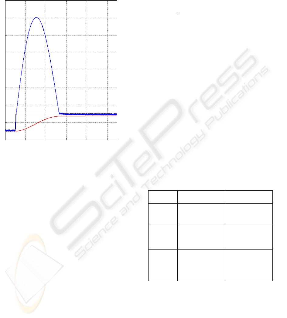
Table 1: Drive switching scheme comparisons.
Control
Scheme
Avantages Disadvantages
Bipolar Good current
control
Faster switching
More heat
More EMI
Unipolar Slower switching
Less heat
Reduced EMI
No current
control
during
regeneration
Hybrid Good current
control
Slower switching
Less heat
Reduced EMI
More complex
circuitry
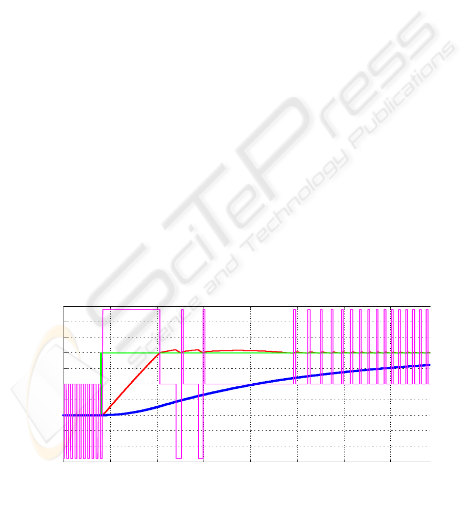
0 0.001 0.002 0.003 0.004 0.005
-20
0
20
40
60
80
100
120
140
seconds
Current demand, motor current and speed
i
ω
i
d
Figure 6: Over current during speed reversal with a
unipolar drive and a large motor as id steps from -
10A to +10A and ω chan
g
es slowl
y
from -10 to +10
recirculation of the motor current through FETs 1
and 4. The governing equation is then:
V
av
= [τ/T-1] V
supply
(3)
The problems with unipolar drives arise when
the motor speed needs to be reversed and the
reversed current is established by a voltage reversal
before the rotation direction has time to change. This
happens (in quadrants 2 and 4) as the current
magnitude increases when the supply is placed
across the motor, but current still increases (at a
slower rate) when recirculating as the back emf is
now assisting the current. The result is a continual
increase in the current until the motor slows and
reverses. Currents of 40A have been measured
(immediately before destruction) in a commercial IC
rated for 3A in quadrants 1 and 3. The effect has
been simulated for a large motor and the results
presented in fig.6. The mechanism for this is found
from the DC motor equations:
V
a
= Ri + L di/dt + k
ω
(4)
Γ
= ki (5)
where
ω
is the motor speed in rads/s, k
ω
the back
emf of the motor, and
Γ
the torque output by the
motor. When connected to the supply, the armature
voltage V
a
= +V
supply
, and when recirculating the
current, V
a
= 0. Consider a change from negative
speed to positive speed: In quadrant 3 the speed is
still negative while the current has become positive,
so when V
a
= 0, the equation 4 becomes:
di/dt = -[kω + Ri]/L (6)
Since ω is large and negative, the current magnitude
will increase during the recirculate period until the
back emf falls to the voltage drop across the
resistance in the current recirculation loop. Equality
occurs when k
ω
= -Ri or
Γ
= -k
2
ω
(7)
This is shown as the dashed line in the 4 quadrant
torque speed plot in fig.5(a).
3 HYBRID SWITCH CONTROL
The novel approach adopted Dunlop and Cree
(1997) is to switch between bipolar and unipolar
control modes as required. The current through the
motor is measured and used to switch from unipolar
mode (cross hatched area in fig.5a) to bipolar mode
when operation moves into the diagonally hatched
area shown in quadrants 2 and 4 of fig.5(a). The
detailed switching operation is illustrated in fig. 7
for a step change in demand current from -10A to
+10A for the same large motor used for fig.6. Notice
ICINCO 2004 - INTELLIGENT CONTROL SYSTEMS AND OPTIMIZATION
44
0
0.005
0.01
0.015
0.02
0.025
0.03
0.035
0
-25
-20
-15
-10
-5
0
5
10
15
20
25
Figure 7: The rapidly switching line represents the motor drive voltage in response to the step reversal in
current demand, the sloping line from -10A to +10A is the motor current, and the wide line from -10 to
+10rads/s is the motor speed.
that the current is fully controlled and that not much
extra bipolar switching is required. The advantages
and disadvantages of the 3 switching modes are
listed in table 1.
The hardware used did not switch both sides at
the same time so the negative voltage step changes
were limited to V
supply
at any one time rather than
2V
supply
for the bipolar drive. Software control can
apply this to all bipolar drives and reduce
electromagnetic interference from the drive.
The application of this hybrid switching
technique to the hand precluded fast measurements
of the motor current which changed very rapidly in
the small motors that have low values of motor
inductance L and relatively high resistance R. Such
rapid current changes would require specialized
hardware to track and control the current as was
done by Dunlop and Cree. It would also need to
operate an order of magnitude faster than for the
larger motors tested with the hardware.
In order to reduce the hardware and heating
requirements in the walker and hand, a model of the
DC motor was used to calculate the motor voltage
required for a given speed state and for the
maximum torque available to change that speed. The
maximum allowable current through the motor is
used to achieve the speed change and that value
must not be exceeded or excessive heating can
destroy the motor. Software is then used to switch
from unipolar driving to bipolar operation as the
motor starts regenerating i.e. operating within
diagonal hatched area in quadrants 2 and 4 in
fig.5(a). As shown in fig.4, the output of the PWM is
applied to FETs 1 and 3, while FETs 2 and 4 can be
driven high or low to set the current direction for a
unipolar drive depending on whether the signal is
connected to logic 1 or 0 by software inside the
CY8C6643 PSoC processor (programmable system
on a chip c.f. Cypress Microsystems). When a
bipolar drive is needed, the PWM is inverted and
applied to FETs 2 and 4. Revision to a unipolar drive
is simply a matter of by passing the inverted PWM
signal and setting the processor output to 0 or 1 for
FETs 2 and 4.
4 MODEL CONTROL
It is desirable to avoid using extra hardware for the
direct measurement of the current in the motors.
This lead to the development of model control for
the 11 DC motors in the dexterous hand. A Simulink
model of the DC motor used in the hand (a
Minimotor 1016 012G) is shown in fig.8. The
leadscrew driven linkages in the finger have a slight
effect on the motor and gearbox, and almost none
during regenerative braking as plain lead screws are
not easily back drive. The main effect is the motor
and gearbox inertia. The basic DC model includes
the thermal power output by the armature resistance,
and the effect of brush and bearing friction. This
friction is overcome by the specified “no load”
current but, as seen from equation 5, the no load
current is zero. In fact the friction must be overcome
and the “no load” current is required to do this. The
friction is modeled as Coulomb friction which
opposes the motion and decreases the torque
INTELLIGENT ELECTRIC DRIVE SYSTEM - A mechatronics approach
45
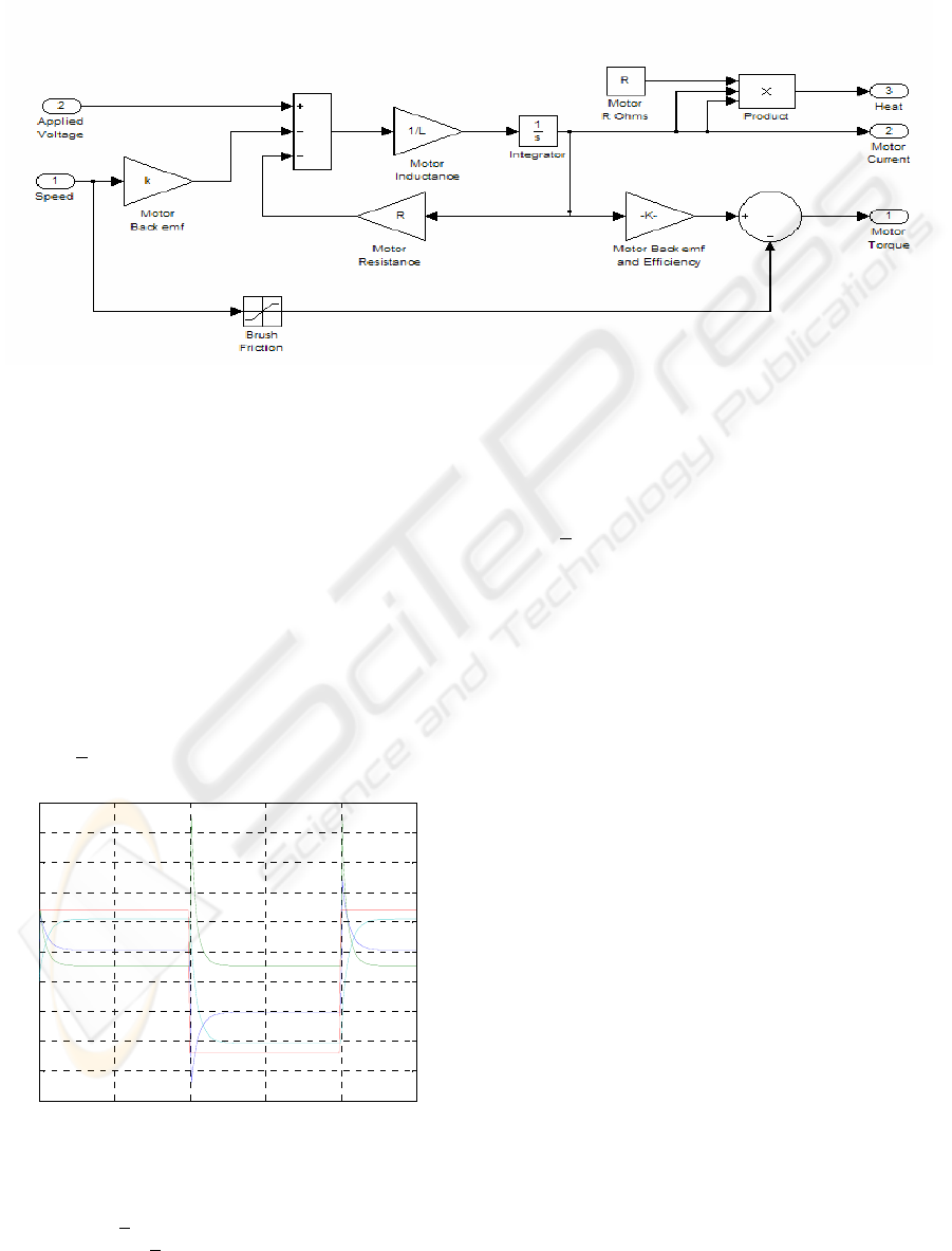
available for motoring in quadrants 1 and 3 of the
torque-speed diagram shown in fig.5(a). The friction
increases the braking during regenerative operation
in quadrants 2 and 4.
Figure 8: Simulink model of the Minimotor includes brush friction to account for no the load torque output.
When the voltage applied to the motor undergoes
changes from +12V to -12V, the motor speed
demand undergoes a step change from 1050 rads/s to
-1050 rads/s as shown in fig.9, and the motor current
peaks at 0.16A. The heating associated with these
peaks during regeneration are a maximum of 2.8W
and the average power is 0.38W for 0.1s reverse
cycling. This is to be compared to the steady state
running value of 0.26W. Thus an increase of 46% of
heat in the motor must be dissipated which equates
to a 46% rise in the temperature above ambient.
This model is placed inside a simple speed
control loop as shown in fig.10. The voltage is
limited to
+12V which is the supply voltage for the
test motor. The rate of change of the voltage applied
to the DC motor is also limited to eliminate
numerical problems associated with both the
Simulink model, and in the PSoC controller which
converts the model voltage into PWM signals for the
H bridge. The short term average of the H bridge
output matches the voltage computed in the speed
control loop. The performance for motor speed
changes
+1000 rads/s is shown in fig.11(a). There
are still large current peaks and the peak power is
2.8W with an average of 0.35W. Some improvement
is needed.
Although this short speed reversing cycle is
somewhat extreme, it does show the various factors
that come into play. The main factor is to limit the
voltage by a known amount relative to the back emf
so that the current can be limited. Rather than
applying a step of voltage to the motor, the voltage
can be changed slowly to match the speed changes.
0 0.05 0.1 0.15 0.2 0.25
-2
-1.5
-1
-0.5
0
0.5
1
1.5
2
2.5
3
seconds
Figure 9: Responses of the control system and load to
rectangular demands for speed change. From the top at
50 ms, the traces are: V
a
the average voltage applied to
the motor (
+12V),
ω
the motor speed in krads/s, i the
motor current (
+50mA), and the heat produced in the
armature windings in Watts.
The Simulink model shown in fig.12 contains a
sub loop to control the voltage demand. This is
simply a model of the electrical part of the motor
with no provision for friction. The derivative of the
shaft position output from the gearbox is used to
derive the speed, and after adjustment for the
gearbox ration, this speed estimate is used in the
velocity feedback loop as well as in the DC motor
model that is used to estimate the motor current that
would result from the application of the voltage
output by the speed error to voltage block in fig.12
(shown as gain and limit blocks in fig.10). The
friction does not need to be modeled in the current
estimator; it is effectively taken care of since the
measured position and derived speed are already
reduced by the friction. The dead zone for the
current limit, gain and summation junction that
ICINCO 2004 - INTELLIGENT CONTROL SYSTEMS AND OPTIMIZATION
46
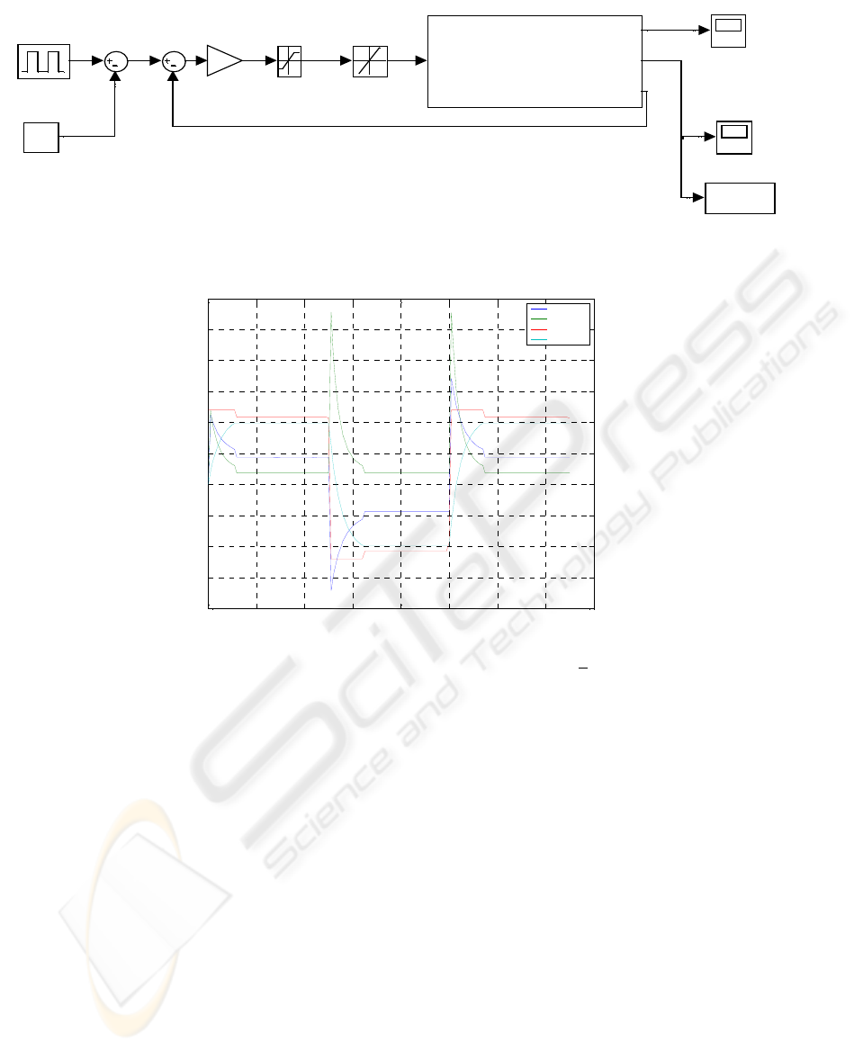
1
V
si m out
To Workspace
Saturation Rate Limiter
Pulse
Generator
Load
Position
Motor Voltage
Load Shaft Rotation rads
Amps Watts Volts rads/s
rads/s
DC Motor + Load Model
1000
Constant
Amps
Figure 10: A finger from the hand showing the 2 DC motors and the control computer and driver PCB.
0 0.02 0.04 0.06 0.08 0.1 0.12 0.14 0.16
-2
-1.5
-1
-0.5
0
0.5
1
1.5
2
2.5
3
seconds
i 0.1A
P W
Va 10V
w rads/s
Figure 11: Speed demand is 0 Æ+1000Æ-1000Æ+1000 rads/s. The drive saturates at
+12V. The peak and average
power dissipation is 3.5W, average of 0.35W using the controller in fig.10. The peak current is 0.17A
follow the estimator are used to decrease the voltage
if excessive motor current would result from directly
applying the demand voltage.
5 DISCUSSION
The use of a velocity control loop within a position
control loop ensures that good positioning
performance can be attained. Hower, large speed
demands translate into large voltages being applied
to the DC motor, and this can give rise to large
currents, and excessive heating. The use of a current
estimator that has the voltage demand and the actual
motor speed as inputs has been shown to provide
good estimates of the current that would occur
should the demand voltage be placed on the actual
motor and load. A dead zone is used to process the
estimated current so that no output occurs unless the
specified motor current limits are exceeded (note
that the limits used here are for inside the hand, not
those specified by Minimotor for a motor with free
air circulation). When the estimated current exceeds
the limits set, then the excess current value is
converted to a voltage that is subtracted from the
demand voltage to give a modified voltage for
application to the actual motor.
6 CONCLUSION
The novel approach used here has proved adequate
for control of the heat build up within a confined
space when several motors are used. Control of the
motor current was crucial for this and as
demonstrated, good control was obtained by using a
model current estimator implemented on a small
control microprocessor. The processor also allowed
for a hybrid switch control of the H bridge to be
used to further reduced the heating. The PSoC
INTELLIGENT ELECTRIC DRIVE SYSTEM - A mechatronics approach
47
controller converts this modified voltage to a PWM
value. It also takes into account the sign of the
voltage and the direction of rotation so that the
appropriate PWM mode can be selected.
REFERENCES
Tal, J., and Persson, E.K., 1978. Pulsewidth modulated
amplifier for DC servo systems. Proc. 7
th
Symp. on
Incremental Motion Control Systems and Devices: DC
motors and control systems, Eds. B.C.Kuo, and J.Tal,
SRL Publishing Co., ISBN 0-918152-02-X, Vol. 1,
ch.11, pp180-200.
Fielding, M. R., and Dunlop, G. R., 2002. Omni
directional hexapod walking and efficient gaits using
restrictedness, Proc 5
th
Int. Conf. on Clinbing and
Walking Robots. ISBN 1-8600-5838-06, pp 501-508.
Fielding, M. R., and Dunlop, G. R., 2004. Omni
directional hexapod walking and efficient gaits using
restrictedness. Accepted for IJRR.
Dunlop, G. R., and Cree, A., 1997. A four quadrant
current driver for direct digital control of a DC motor.
Proc. 26
th
Symp. on Incremental Motion Control
Systems and Devices, Ed B.C.Kuo, SRL Publishing
Co., ISBN 0-931538-20-3, pp 143-150.
Cypress Microsystems www.cypressmicro.com
si m ou t
To Workspace
Speed rads/s Voltage
Speed to Voltage
Speed Required
Speed
Demand
Load
Position
Output SpeedMotor Speed
Gearbox
-K-
Gain
du/dt
Derivative
Motor Voltage
Amps Watts Volts rads/s
Load Shaft Rotation rads
DC Motor + Load Output Model
Motor Speed
Motor Voltage
Motor Am ps
DC Motor + Load Model
Current Limit
Amps
Figure 12: A finger from the hand showing the 2 DC motors and the control computer and driver PCB.
0 0.02 0.04 0.06 0.08 0.1 0.12 0.14 0.16
-1.5
-1
-0.5
0
0.5
1
1.5
seconds
i 0.1A
P W
Va 10V
w rads/s
Figure 13: Speed demand is 0 Æ+1000Æ-1000Æ+1000 rads/s. The voltage drive saturates at
+12V. The peak e
power dissipation is 0.45W with an average of 0.25W for the controller in fig.12. The peak current is around 0.07A so
current control is greatly enhanced.
ICINCO 2004 - INTELLIGENT CONTROL SYSTEMS AND OPTIMIZATION
48
