Neuro-Controller with Simultaneous Perturbation
for Robot Arm
–Learning of Kinematics
and Dynamics without Jacobian
Yutaka Maeda
1
, Nobutaka Kitajima
1
, Tsubasa Inagaki
1
and Hidenori Onishi
1
Kansai University, Faculty of Engineering,
Department of Electrical Engineering and Computer Science
Abstract. We report two control schemes for a two-link robot arm system using
a neuro-controller. We adopted the simultaneous perturbation learning rule for
a neuro-controller. Ordinary gradient type of learning rule uses Jacobian of the
objective system in a direct control scheme by a neural network. However, the
learning rule proposed here requires only two values of an error function. Without
Jacobian or related information of the objective robot arm, the neuro-controller
can learn an inverse of robot kinematics and dynamics, simultaneously. Some
results are shown.
1 Introduction
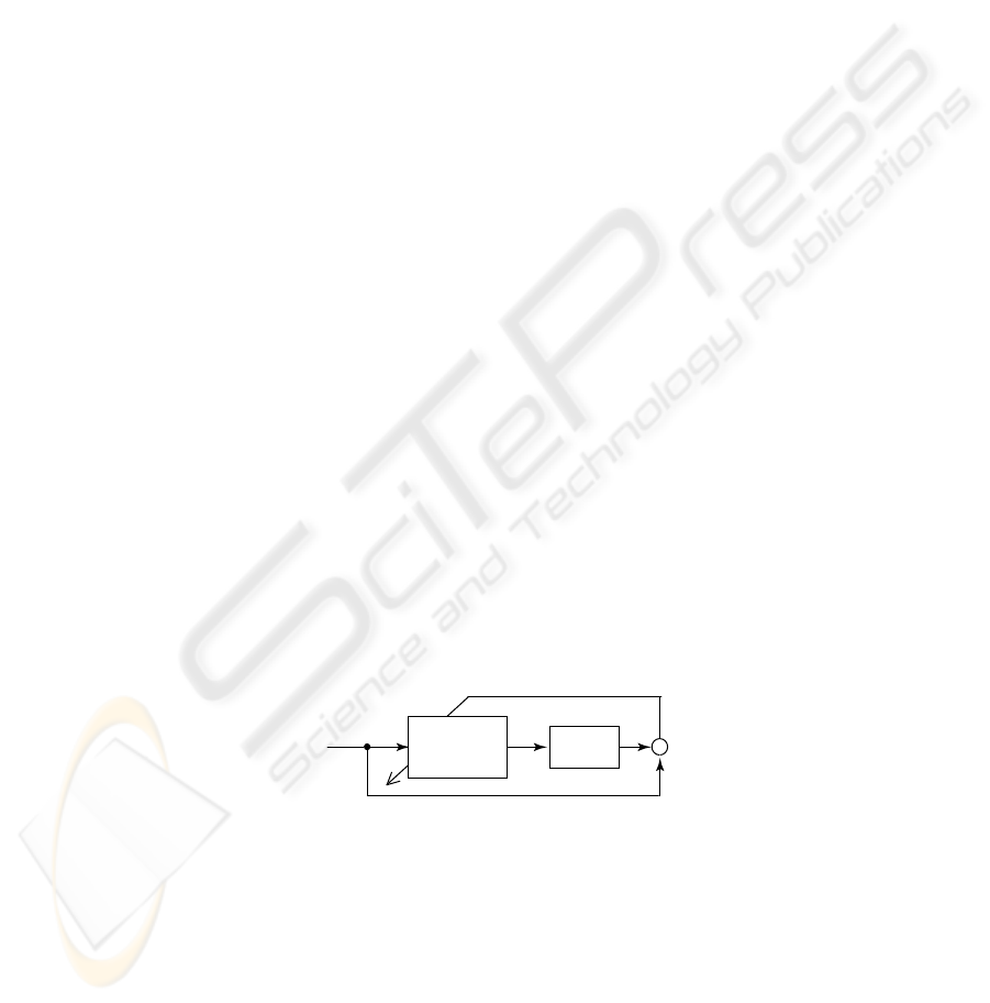
Neuro-Controller (NC) by a direct inverse control scheme (see Fig.1) is a promising
approach for non-linear control problems. When we use a gradient type of learning
rule such as the back-propagation method for the NC, it is essential to know Jacobian
or related information on an objective plant[1]. However, it is generally impossible or
very difficult to know the Jacobian especially for a nonlinear objective.
Neuro-
controller
Plant
+
-
y
u
J(w)
w
f (u)
y
d
Desired
output
Output
Error function
Fig. 1. A basic scheme for a neuro-controller.
In this paper, we propose control schemes by neural networks (NNs) using the si-
multaneous perturbation learning rule for a two link robot arm system. This learning
rule does not directly require a derivative of an error function but only values of the
Maeda Y., Kitajima N., Inagaki T. and Onishi H. (2004).
Neuro-Controller with Simultaneous Perturbation for Robot Arm Learning of Kinematics and Dynamics without Jacobian.
In Proceedings of the First International Workshop on Artificial Neural Networks: Data Preparation Techniques and Application Development, pages
16-22
DOI: 10.5220/0001149200160022
Copyright
c
SciTePress
2
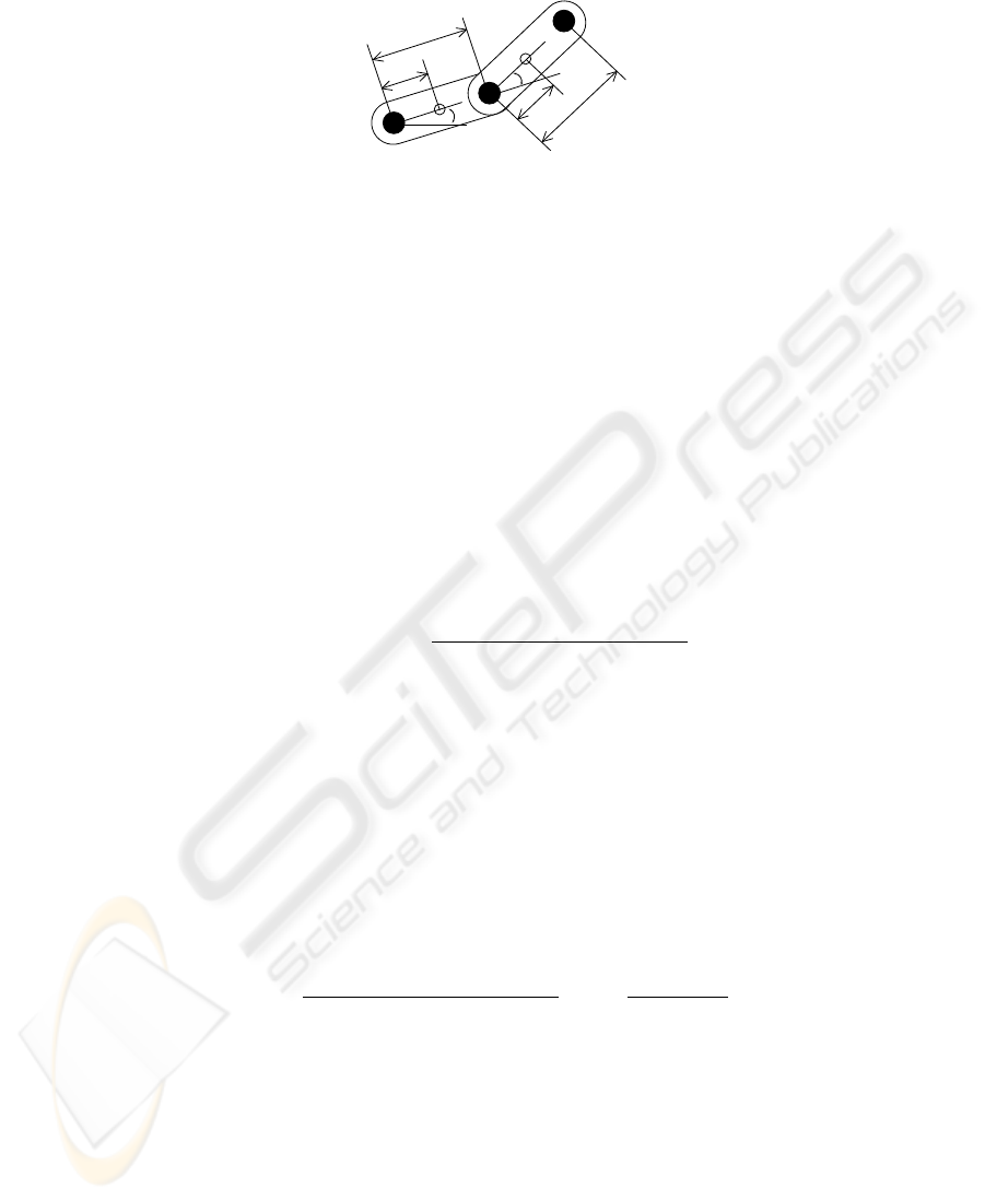
l
link-1
link-2
1
l
2
r
1
r
1
ǰ
2
ǰ
Top
Fig. 2. Two link robot arm system.
error function itself. Therefore, without knowing Jacobian of the objective system, we
can design a direct neuro-controller and then the neuro-controller can learn a robot
kinematics and a dynamics simultaneously. Moreover, the NC is able to adapt changing
environment through learning.
2 Simultaneous Perturbation for Neuro-Controller
The simultaneous perturbation(SP) and its applications are widely reported[1–4]. We
explain the SP learning rule with a sign vector for NCs. Now let w, J(·) and u be a
weight vector of the NC including thresholds, an error function and an input for the
robot arm, respectively. The learning rule via the SP is as follows;
w
t+1
= w
t
− α
J(u(w
t
+ cs
t
)) − J(u(w
t
))
c
s
t
(1)
Where, α and c are a positive learning coefficient to adjust a magnitude of a modifying
quantity and a magnitude of a perturbation, respectively. s denotes a sign vector whose
components are +1 or -1. Moreover, t is iteration.
Note that only two values of the error function J(u(w)) and J(u(w + cs)) are
used to update the weights in the neural network. Any information about the objective
plant such as Jacobian does not have to be required in this learning rule. Therefore,
this learning rule is easily applicable to the direct control scheme by NCs for a plant
including unknown and/or unmodeled factors.
It is known that the learning rule has the following property[1]. That is, the learning
rule is a kind of stochastic gradient learning rule.
E
µ
J(u(w
t
+ cs
t
)) − J(u(w
t
))
c
s
t
=
∂J (u(w
t
))
∂w
(2)
Note that the SP learning rule is not a merely expansion of the ordinary finite dif-
ference approximation. In our case, we have to adjust plural parameters, that is, weight
values in the NC. The number of the weights is relatively large. If we simply use the
finite difference, we have to know many values of the error J for all weights to update.
On the other hand, the SP method requires only two values of the error, even if the
number of the weights of the NC is large.
17
3 Control Scheme 1
3.1 Configuration
We consider the two-link robot arm (see Fig.2) as an objective nonlinear plant. Now our
problem is to control the end of the link-2 of the robot arm in Fig.2. Then purpose of
the NC is to generate proper torque values for the two links.
Fig.3 shows overall configuration of the robot system using a NC. For one trial, the
NC with certain weights outputs a series of torque signals to the robot arm. Then we
have a locus. Thus we can obtain a value of the error function as follows;
J(u(w)) =
X
i
¡
(x
i
− x
di
)
2
+ (y
i
− y
di
)
2
¢
(3)
Where, x
i
, y
i
and x
di
, y
di
denote actual position of the top and its desired position,
respectively. With the perturbation, we make a trial again and obtain a value of the error.
Using these two values and Eq.(1), we update the weights. We repeat this procedure.
d d
x , y
x, y
Simultaneous
perturbation
RNN
Robot arm
Modify weights
desired
position
torque
τ1, τ2
position
of the top
+
-
θ , θ , θ
& &&
state of the arm:
Fig. 3. Overall configuration of control scheme 1.
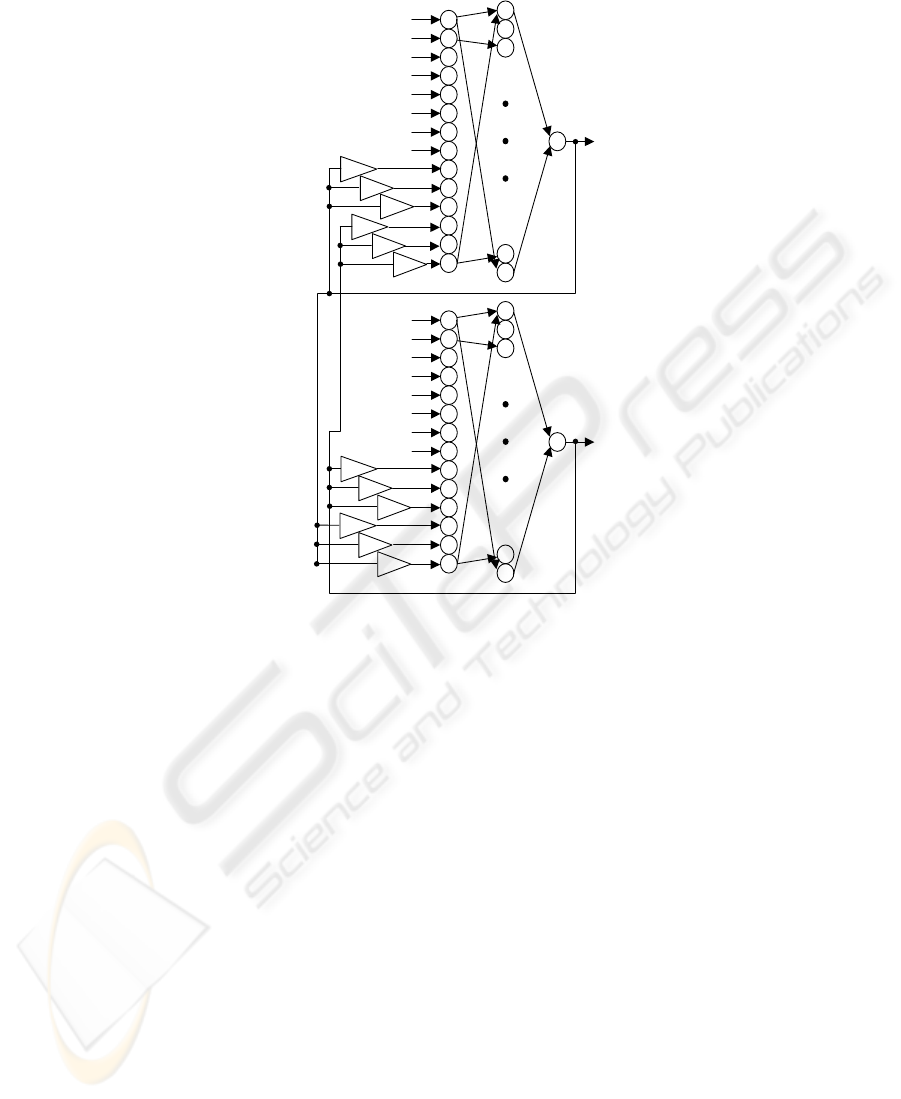
The objective plant has a dynamics. Therefore, a simple multi-layered neural net-
work cannot control the plant, since the network does not have any dynamics. Basically,
the NC consists of two multi-layered neural networks shown in Fig.4. However, the
neural networks have time-delayed feedback inputs from outputs of the networks. This
feedback gives dynamics to the networks.
Both networks have 14 neurons in input layer, 20 neurons in middle layer, 1 neuron
in output layer. The NC uses desired position, angles θ
1
and θ
2
, velocities of the angles
˙
θ
1
and
˙
θ
2
, accelerations of the angles
¨
θ
1
and
¨
θ
2
, time-delayed outputs of the network as
inputs. Outputs correspond to torque of the link-1 and the link-2.
18
1ðt
x
y
1
q
2
q
z
-1
z
-1
z
-1
z
-1
z
-1
z
-1
z
-1
z
-1
z
-1
z
-1
z
-1
z
-1
2
q
1
q
2
q
1
q
x
y
1
q
2
q
2
q
1
q
2
q
1
q
t
1
t
2
d
d
d
d
Fig. 4. Neuro-controller used here.
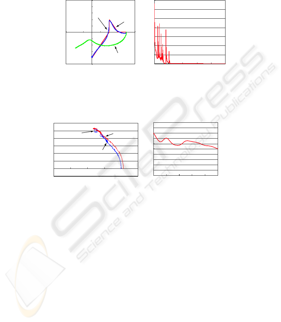
3.2 Result
We consider some practical tasks for the system. Using a proper model of the robot arm,
we have a simulation result(see Fig.5) for locus control. Then the learning coefficient
α = 0.0005 and the perturbation c = 0.00008. After 10000 times learning, locus of the
top is close to a desired one. The error value decreases as iteration proceeds.
Next, we consider a movement of the top to a certain point. Fig.6 shows a result
of the actual robot arm. After pre-training by simulation, the NC is used for the actual
system. Then the learning process and operations themselves are carried out simultane-
ously. α = 0.01 and c = 0.05. After 10 times learning by the actual system, the top
moves to a target point. Before the learning, the top stopped at a point that is different
from the target. As is shown in Fig.6(b), the error decreases.
The learning coefficient α and the perturbation c are determined empirically. How-
ever, the learning rule is not so sensitive to these values.
19
㪄㪇 㪅㪌
㪄㪇 㪅㪋
㪄㪇 㪅㪊
㪄㪇 㪅㪉
㪄㪇 㪅㪈
㪇
㪇㪅㪈
㪇㪅㪉
㪇㪅㪊
㪇㪅㪋
㪇㪅㪌
㪄㪇 㪅㪊 㪄㪇 㪅㪈 㪇㪅㪈 㪇㪅㪊 㪇㪅㪌
x-axis[m]
y-axis[m]
㪇
㪌
㪈㪇
㪈㪌
㪉㪇
㪉㪌
㪊㪇
㪊㪌
㪇 㪉㪇㪇㪇 㪋㪇㪇㪇 㪍㪇㪇㪇 㪏㪇㪇㪇 㪈㪇㪇㪇㪇
Desired locus
Before learning
After learning
Iteration
Squared error
(a) Loci before and after learning. (b) Change of squared error.
Fig. 5. Simulation result for a locus.
㪄㪇㪅㪇㪌
㪇
㪇㪅㪇㪌
㪇㪅㪈
㪇㪅㪈㪌
㪇㪅㪉
㪇㪅㪉㪌
㪇㪅㪊
㪇 㪇㪅㪈 㪇㪅㪉 㪇㪅㪊 㪇㪅㪋 㪇㪅㪌
x-axis[m]
y-axis[m]
㪇㪅㪇
㪇㪅㪉
㪇㪅㪋
㪇㪅㪍
㪇㪅㪏
㪈㪅㪇
㪈㪅㪉
㪈㪅㪋
㪈㪅㪍
㪈㪅㪏
㪉㪅㪇
㪇 㪉 㪋 㪍 㪏 㪈㪇
Iteration
squarred error
Target
After learning
Before learning
(a) Loci before and after learning to target point . (b) Change of squared error.
Fig. 6. Experimental result for a target point.
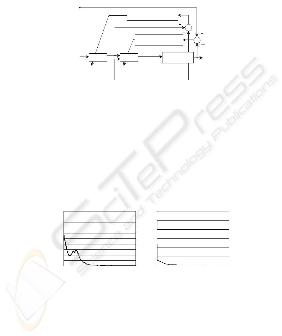
4 Control Scheme 2
4.1 Configuration
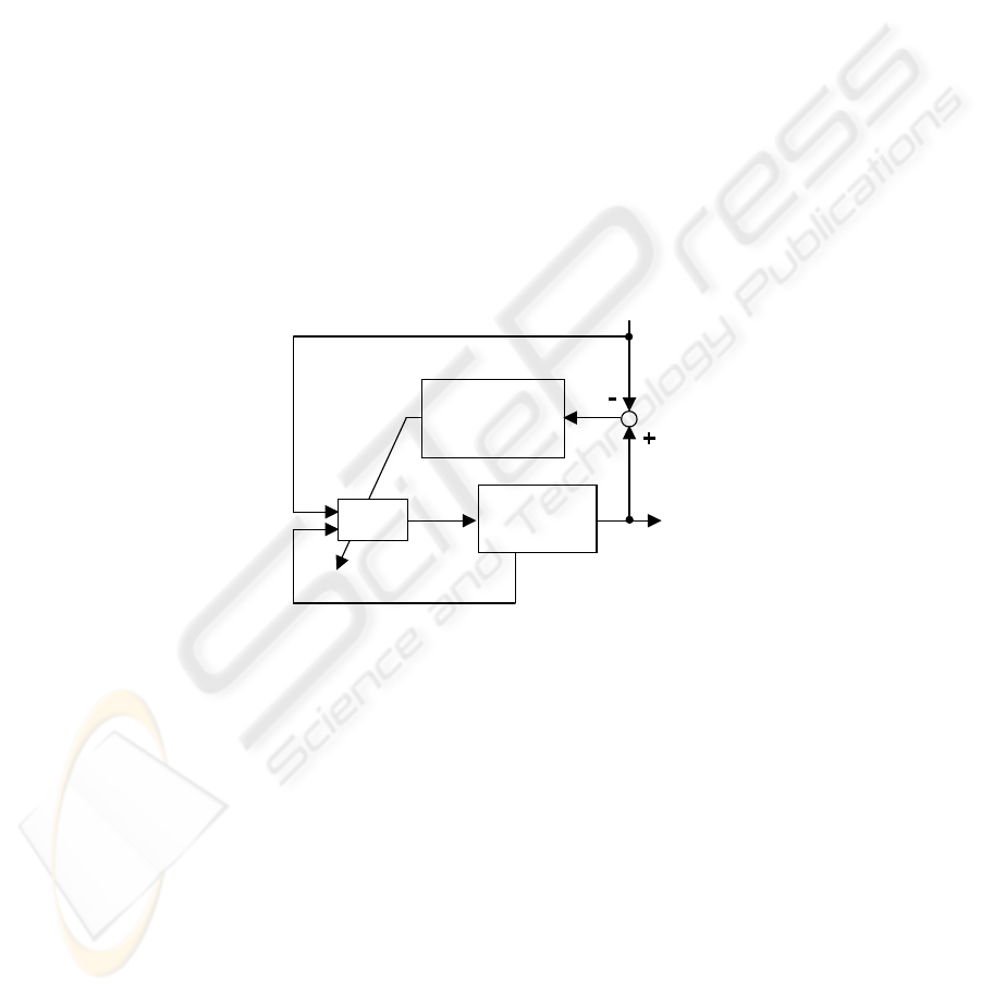
Next, we consider more complicated configuration to handle the problem. We prepare
two NNs. One neural network is for kinematics. Inputs of the network are desired po-
sition of the top of the arm in xy coordinate. Outputs are angles for the two arms. The
neural network must learn an inverse kinematics of the robot arm system. The second
neural network is a recurrent neural network (RNN). Inputs of the network are the an-
gles of the arm, that is, the outputs of the first network and state of the objective robot
arm. Outputs are torque values for the two links. The second network must learn an
inverse dynamics of the plant. The configuration is depicted in Fig.7.
In this case, it is difficult to carry out the learning of these two NNs, simultaneously.
As same as the previous configuration, if we use an ordinary gradient method to update
20
+
-
θ
1
, θ
2
θ , θ , θ
& &&
RNNNN
x, y
state of the arm:
Robot arm
τ1, τ2
xd, yd
desired position
simultaneous perturbation
learning rule
simultaneous perturbation
learning rule
-
+
torque
angle
position
of the top
Modify weights
Modify weights
angle
Fig. 7. Overall configuration of control scheme 2.
the weights in these two networks, it is essential to know the Jacobian of the plant. On
the hand, our approach does not require the information.
The first NN for the kinematics updates their weights based on the error defined by
the output angles and the actual angles of the two links of the robot arm. Moreover, the
second RNN learns the dynamics using the error defined by the actual xy position of
the robot arm and the corresponding desired position.
4.2 Simulation result
㪇
㪌
㪈㪇
㪈㪌
㪉㪇
㪉㪌
㪊㪇
㪊㪌
㪋㪇
㪋㪌
㪌㪇
㪇 㪈㪇㪇㪇 㪉㪇㪇㪇 㪊㪇㪇㪇
(a) Error for inverse kinematics
Iteration
Squared error
㪇
㪈㪇
㪉㪇
㪊㪇
㪋㪇
㪌㪇
㪍㪇
㪇 㪈㪇㪇㪇 㪉㪇㪇㪇 㪊㪇㪇㪇
(b) Error for inverse dynamics
Iteration
Squared error
Fig. 8. Change of errors.
We consider a task to move the top of the arm to a certain point using the control scheme
2.
21
㪇㪅㪇
㪇㪅㪈
㪇㪅㪉
㪇㪅㪊
㪇㪅㪋
㪇㪅㪇 㪌㪅㪇 㪈㪇㪅㪇 㪈㪌㪅㪇 㪉㪇㪅㪇
x position[m]
Time[sec]
desired position
before learning
after learning
㪄㪇㪅㪋
㪄㪇㪅㪊
㪄㪇㪅㪉
㪄㪇㪅㪈
㪇㪅㪇
㪇㪅㪈
㪇㪅㪉
㪇㪅㪊
㪇㪅㪋
㪇㪅㪇 㪌㪅㪇 㪈㪇㪅㪇 㪈㪌㪅㪇 㪉㪇㪅㪇
y position[m]
Time[sec]
desired position
before learning
after learning
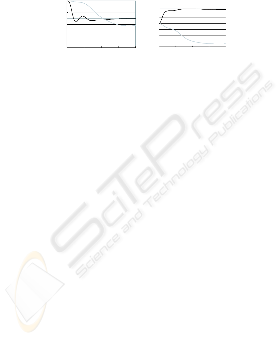
Fig. 9. Simulation result.
Fig.8 shows changes of the errors for the kinematics and the dynamics. This simu-
lation result reveals that 1000 learning gives proper accuracy to move the top of the arm
to the desired position. Then, α = 0.0008 and c = 0.0003.
Fig.9 is xy position of the top. After 3000 learning, the top moves to the desired
position. This shows that the first NN and the second NN learn the inverse kinematics
and the inverse dynamics properly.
5 Conclusion
This paper describes two control schemes for the two link robot arm. In these control
schemes, the NNs learn the inverse of the kinematics and the dynamics of the objective
robot system without Jacobian of the plant. The simultaneous perturbation learning rule
makes this possible.
Acknowledgement
This work was financially supported by Grant-in-Aid for Scientific Research(No.16500142)
of the Ministry of Education, Culture, Sports, Science and Technology of Japan.
References
1. Maeda, Y., deFigueiredo, R.J.P.: Learning Rules for Neuro-Controller via Simultaneous Per-
turbation. IEEE trans. on Neural Networks, 8 (1997) 1119–1130
2. Spall, J.C.: Multivariable stochastic approximation using a simultaneous perturbation gradient
approximation. IEEE Trans. Autom. Control, AC-37 (1992) 332–341
3. Cauwenberghs, G.: A fast stochastic error-descent algorithm for supervised learning and op-
timization. in S.J.Hanson, J.D.Cowan and C.Lee(eds.), Advances in neural information pro-
cessing systems 5, Morgan Kaufmann Publisher. (1993) 244–251
4. Maeda, Y., Hirano, H., Kanata, Y.: A learning rule of neural networks via simultaneous per-
turbation and its hardware implementation. Neural Networks, 8 (1995) 251-259
22
