
Enlarging Training Sets for Neural Networks
R. Gil-Pita
?
, P. Jarabo-Amores, M. Rosa-Zurera, and F. L
´
opez-Ferreras
Departamento de Teor
´
ıa de la Se
˜
nal y Comunicaciones,
Escuela Polit
´
ecnica Superior, Universidad de Alcal
´
a
Ctra. Madrid-Barcelona, km. 33.600, 28805, Alcal
´
a de Henares - Madrid (SPAIN).
Abstract. A study is presented to compare the performance of multilayer per-
ceptrons, radial basis function networks, and probabilistic neural networks for
classification. In many classification problems, probabilistic neural networks have
outperformed other neural classifiers. Unfortunately, with this kind of networks,
the number of required operations to classify one pattern directly depends on
the number of training patterns. This excessive computational cost makes this
method difficult to be implemented in many real time applications. On the con-
trary, multilayer perceptrons have a reduced computational cost after training, but
the required training set size to achieve low error rates is generally high. In this
paper we propose an alternative method for training multilayer perceptrons, us-
ing data knowledge derived from the probabilistic neural network theory. Once
the probability density functions have been estimated by the probabilistic neural
network, a new training set can be generated using these estimated probability
density functions. Results demonstrate that a multilayer perceptron trained with
this enlarged training set achieves results equally good than those obtained with
a probabilistic neural network, but with a lower computational cost.
1 Introduction
A study is presented to compare the performance of three types of artificial neural net-
works (ANNs), namely, multilayer perceptron (MLP), radial basis function network
(RBFN), and probabilistic neural network (PNN) for classification. Two experiments
are defined in order to asses the performance of the methods. In both experiments, the
extracted features from signals are used as inputs to the classifiers: MLP, RBFN, and
PNN for pattern recognition. Characteristic parameters like number of nodes in the
hidden layer of MLP, and number of radial basis functions of RBFN, are optimized in
terms of error rate. For each experiment, ANNs are trained with a subset of the available
experimental data. ANNs are tested using the remaining set of data.
In many classification problems, PNNs have outperformed other neural classifiers.
Unfortunately, with this kind of networks, the number of required operations to clas-
sify one pattern directly depends on the number of training patterns. This excessive
computational cost makes this method difficult to be implemented in many real time
?
This work has been supported by the “Consejer
´
ıa de Educaci
´
on de la Comunidad de Madrid”
(SPAIN), under Project 07T/0036/2003 1
Gil-Pita R., Jarabo-Amores P., Rosa-Zurera M. and López-Ferreras F. (2004).
Enlarging Training Sets for Neural Networks.
In Proceedings of the First International Workshop on Artificial Neural Networks: Data Preparation Techniques and Application Development, pages
23-31
DOI: 10.5220/0001149800230031
Copyright
c
SciTePress

applications. On the contrary, the number of operations required to classify one pattern
using MLPs uses to be low, due to the characteristics of this kind of network.
In this paper we propose an alternative method for training MLPs, using data knowl-
edge derived from the PNN theory. Once the probability density functions (PDFs) have
been estimated by the PNN, a new training set can be generated using these estimated
PDFs. Results demonstrate that a MLP trained with this enlarged training set achieves
results equally good than those obtained with PNNs, but with a very low computational
cost.
2 Studied Neural Networks
In this section a short review of three kinds of neural networks is carried out. The neural
networks reviewed in this paper are the MLP, the RBFN and the PNN.
2.1 Multilayer perceptron
The Perceptron was developed by F. Rosenblatt [1] in the 1950s for optical charac-
ter recognition. The Perceptron has multiple inputs fully connected to an output layer
with multiple outputs. Each output y
j
is the result of applying the linear combination
of the inputs to a non linear function called activation function. Multilayer Perceptrons
(MLPs) extend the Perceptron by cascading one or more extra layers of processing
elements. These extra layers are called hidden layers, since their elements are not con-
nected directly to the external world.
Cybenko’s theorem [2] states that any continuous function f : R
n
→ R can be ap-
proximated with any degree of precision by a network of sigmoid functions. Therefore
we chose an MLP with one hidden layer using the sigmoidal function given in (1) as
the activation function.
L(x) =
1
1 + exp(−x)
(1)
In this paper, the MLPs are trained using the Levenberg-Marquardt algorithm [3].
The error surface for the given problem has many local minima. Consequently, each
experiment was repeated 10 times, and the best network in terms of error rate was
selected.
2.2 Radial basis function network
In Radial Basis Function Networks, the function associated with the hidden units (radial
basis function) is usually the multivariate normal function, which is described by (2) for
a given hidden unit i and a given pattern x.
G
i
(x) =
|C
i
|
−1
2
(2π)
n
2
exp(−kx − t
i
k
2
C
i
) (2)
24

C
i
can be set to a scalar multiple of the identity matrix, to a diagonal matrix with
different diagonal elements, or to a non-diagonal matrix. We have set C
i
to a scalar
multiple of the identity matrix.
To train the RBFNs, we applied a three-phased learning strategy [4][5][6]:
1. The centers of the radial basis functions are determined by fitting a Gaussian mix-
ture model with circular covariances using the EM algorithm. The mixture model
is initialized using a small number of iterations of the k-means algorithm.
2. The basis function widths are set to the maximum squared inter-center distance.
3. The output weights can be determined using the LMS algorithm.
Again, each training run was repeated 10 times, and the best case in terms of error
rate was selected. During training, the test set was used to monitor the learning progress
and consequently to determine when to stop the learning process.
2.3 Probabilistic neural network
PNN or probabilistic neural network is Specht’s [7] term for kernel discriminant analy-
sis. It is a normalized RBFN in which there is a hidden unit centered at every training
pattern. The output weights are 1 or 0. For each hidden unit, a weight of 1 is used for
the connection going to the output the pattern belongs to, while all other connections
are given weights of 0. Each output unit p calculates its activation for a test pattern x as
follows:
f
p
(x) =
1
L − K
L
X
i=K
exp
µ
−
P
N
j=1
(x(j)−c
i
(j))
2
2h
i
(j)
2
(2π)
N
2
Q
N
j=1
h
i
(j)
(3)
where N is the input dimension, the hidden units K to L participate in the spe-
cific class p, c
i
is the i-th training pattern and h
i
are the smoothing parameters, which
correspond with the square root of the diagonal of the covariance matrix of the Gaus-
sian kernel function. It can be demonstrated than each output of the PNN is a universal
estimator of the PDF of each class.
To adapt the kernel function to the data distribution, we propose the use of different
values of the smoothing parameter, depending on the coordinate. For a given training set
{x
1
, x
2
, . . . , x
N
}, we calculate the smoothing parameter along each coordinate, h
i
(j),
for each training sample, x
i
= (x
i
(1), x
i
(2), . . . , x
i
(n)), with (4):
h
i
(j) =
1
K − 1
K
X
k=1,k6=i
|x
ij
− x
kj
| (4)
3 Improving Neural Network Performance
In many applications, PNNs obtain lowest error rates, but with a high computational
cost. The number of operations required to classify one pattern depends directly on
25

the training set size. The other neural solutions have a structure independent of the
training set size. The objective of this paper is the proposal of a classification method
that achieves error rates as low as PNNs, with the low computational cost of other neural
classifiers. Once the PDFs attached to the PNN have been estimated, new synthetic
training data are generated in accordance with these estimated PDFs. The performance
of neural networks trained using the synthetic training sets matches or even surpasses
the best performance of PNNs, at lower computational costs after training.
The idea of extending the training set with synthetic samples has been presented in
the literature several times. Abu-Mostafa [8] proposed the use of auxiliary information
(’hints’) about the target function to guide the learning process. Niyogi, Girosi and
Poggio [9] generated synthetic data by creating mirror images of the training samples.
We propose a fundamentally different method, in so far as no additional information
about the data is necessary, and there are no limits to the size of the synthetic training
data set. It is based on estimating the PDF of a given class. By using the estimation of
the PDF to generate the additional training data, all possible data hints are used without
prior knowledge of the training data properties.
As described in Subsection 2.3, the estimator of the PDF is a combination of Gaus-
sian functions. So, it is relatively simple to generate any number of patterns with the
estimated PDF. To generate each new pattern, the following procedure is applied:
1. A class is randomly selected, taking into account all the classes are equally likely.
2. After a class is selected, a Gaussian function is randomly selected from those com-
bined to estimate the class PDF.
3. The new pattern is generated as a Gaussian vector with the selected Gaussian func-
tion.
Thus we can increase the training set sufficiently and train the MLP with these synthetic
data. Using the kernel method described in Subsection 2.3 to estimate the PDFs, each
training set size has been virtually multiplied by a factor of 40 (with this factor we hoped
for a substantial improvement). It is obvious that the computational costs incurred with
the PDF estimations and training using the new training sets increase considerably; but
the reduction of the error rate and the low computational costs for the classification of
one pattern after training are significant enough to outweigh this disadvantage.
Once the enlarged training sets have been generated, we have trained MLPs using
the Levenberg-Marquardt algorithm [3]. Each training has been repeated 10 times, and
the best case in terms of error rate was selected. During training, the test set was used to
monitor the learning progress and consequently to determine when to stop the learning
process.
4 Experiment 1: Three Gaussian Classes
A training set has been created composed of three different classes (C
1
, C
2
, C
3
). All
three classes are associated to a 8-dimensional multivariate gaussian with a mean vector
equal to zero and with a covariance matrix equal to the identity matrix multiplied by
σ
2
. This is equivalent to a 8-dimensional vector z in which each component z
i
is an
26

independent gaussian random variable with zero mean and variance equal to σ
2
. The
PDF of each vector is described in (5).
f(z|C
i
) =
1
√
2πσ
8
i
exp(
z · z
T
−2σ
16
i
) (5)
where σ
1
= 1, σ
2
= 2 and σ
3
= 3. In this case the optimal classifier can be
calculated by the Maximum a Posteriori criterium. So, for a given observation vector
z a decision in favor of class C
i
is taken, if f(z|C
i
) > f(z|C
j
) for all j 6= i. This
condition can also be expressed with (6).
|z| > 4
σ
j
· σ
i
q
σ
2
j
− σ
2
i
·
r
log(
σ
j
σi
) (6)
Three regions corresponding to the three classes are delimited by two hyper-spheres.
Therefore, the optimum classifier is obtained by calculating the magnitude of the ob-
servation. The error probability associated to this optimum classifier is 20.30%.
For the first experiment, that tries to approximate the optimum classifier, two subsets
were used: a training set composed of 300 signals (100 per class), randomly generated
using the probability density functions described in (5), and a test set, composed of
1000 profiles of each class. The test set serves two purposes: during training it helps
to evaluate progress, whereas after training it is used to assess the classifier’s quality
(validation set).
In order to study the dependence of performance on the parameters of the classifi-
cation methods, we vary the size of the networks:
– For the MLPs trained with the original data set, the number of neurons in the hidden
layer varies from 4 to 80 in increments of 4 for each training set.
– For the RBFNs, the number of radial basis functions takes the values from 10 to
150 in steps of 10.
– The enlarged training set has 12000 samples. For the MLPs trained with the en-
larged data set, the number of neurons in the hidden layer varies from 4 to 60 in
increments of 4 for each training set.
Table 1 shows the results on error rate and computational complexity, obtained ap-
plying the different neural classifiers studied in this paper. The error rate is expressed
by the average number of errors classifying the test set, and the computational com-
plexity is expressed by the number of trivial operations needed to classify one pattern
after training. Only the network sizes which achieved the best error rates are consid-
ered. The best results are obtained by a MLP with 68 hidden neurons and a RBFN with
60 radial basis functions. The best MLP trained with the enlarged training set has 24
hidden neurons.
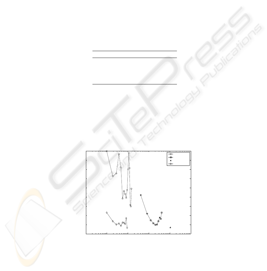
Figure 1 shows the achieved error rate vs. the computational complexity for the
methods studied in this paper. Results demonstrate the good performance of the pro-
posed method, which obtains a error rate similar to the best PNN, but with a reduced
computational complexity after training.
27

Table 1. Experiment 1: average error rates and number of operations using the studied methods
Classifier Error rate (%) Operations
MLP 33.27 % 1570
RBFN 32.90 % 1863
PNN 29.93 % 11403
PNN+MLP 30.10 % 558
10
1
10
2
10
3
10
4
10
5
0.28
0.3
0.32
0.34
0.36
0.38
0.4
0.42
Number of Operations
Error Rate
MLP
RBFN
PNN
PNN+MLP
Fig. 1. Experiment 1: error rate and number of operations to classify one pattern
5 Experiment 2: Radar Target Classification
The objective of the second experiment is to study the performance of different High
Range Resolution (HRR) radar target classifiers. For this purpose, a data base con-
taining HRR radar profiles of six types of aircrafts has been used. The assumed target
position is head-on with an azimuth range of 25
o
and elevations of −20
o
to 0
o
in one
degree increments, totaling 1071 radar profiles per class. The length of each profile is
40.
In [10] the influence of the sizes of training and test sets was studied for RBFNs and
MLPs. Training set sizes of 60, 240, 420 and 600 were used. For comparison purposes,
a training set composed of 600 profiles (100 per class), randomly selected from the
original data set, and a test set, composed of 971 profiles of each class have been used.
The test set serves two purposes: during training it helps to evaluate progress, whereas
after training it is used to assess the classifier’s quality (validation set).
Again, we altered the size of the networks in order to study its influence over the
performance of the classifiers:
– For the MLPs trained with the original data set, the number of neurons in the hidden
layer varies from 4 to 64 in increments of 4 for each training set.
– For the RBFNs, the number of radial basis functions takes the values from 30 to
300 in steps of 30.
28
– The enlarged training set has 24000 radar profiles. For the MLPs trained with the
enlarged data set, the number of neurons in the hidden layer varies from 4 to 40 in
increments of 4 for each training set.
The computational complexity is an important issue. With MLP based classifiers
it is low after training, compared with the computational complexity of the RBFN or
PNN. In table 2 we present the performance of the different neural networks studied
in the paper applied to the HRR radar target classification problem, representing both
error rate and computational complexity. The best results are obtained by a MLP with
60 hidden neurons and a RBFN with 150 radial basis functions. The best MLP trained
with the enlarged training set has 40 hidden neurons.
Table 2. Experiment 2: average error rates and number of operations using the studied methods
Classifier Error rate (%) Operations
MLP 4.97 % 5706
RBFN 2.98 % 26556
PNN 2.68 % 106206
PNN+MLP 2.65 % 3806
Figure 2 shows the achieved error rate vs. the computational complexity of the clas-
sifier for the methods studied in this paper. Results obtained with the new classification
method are better than the results obtained with the other methods studied in this paper,
both in error rate and computational cost after training.
10
1
10
2
10
3
10
4
10
5
10
6
0.02
0.03
0.04
0.05
0.06
0.07
0.08
0.09
0.1
0.11
Number of Operations
Error rate
MLP
RBFN
PNN
PNN+MLP
Fig. 2. Experiment 2: error rate and number of operations to classify one pattern
29

6 Conclussions
In this paper, a study is presented to compare the performance of three kinds of neural
networks: MLPs, RBFNs and PNNs. We also present a new strategy that combines the
characteristics of MLPs and PNNs. This strategy uses the estimates of the PDFs of the
classes, obtained from the actually available training data, to generate synthetic patterns
and, therefore, an enlarged training set. These new set is used to train an MLP-based
classifier.
Both the MLP-based classifier and the RBFN-based classifier are a compromise be-
tween computational complexity and error rates. As the error rate decreases, the com-
putational complexity increases, and vice versa. The curves represented in figures 1
and 2 for the MLP-based classifier and the RBFN-based classifier could be seen as
segments of an overall curve that shows the relationship between error rate and com-
putational complexity. This curve shows an indirect proportionality between accuracy
and computational costs until we reach the point of the minimum error rate. From this
point on, increasing the computational effort does not yield better results in terms of
error rate. The part of this curve with low computational complexity corresponds to
the MLP-based classifier. The part with low error rates corresponds to the RBFN-based
classifier.
The performance of the MLP trained with synthetic samples generated from the
estimated PDFs of the respective classes (PNN+MLP) significantly surpasses the results
obtained with the RBFN-based classifiers, and MLP-based classifiers. Better still, this
improvement is achieved in both areas, error rate and computational complexity.
Comparing with the PNN, the proposed method equals the performance of the PNN,
but with a dramatically reduced computational complexity. These gains represent an
important increase in the efficiency.
In summary, we can conclude that the proposed method for increasing the size of
the training set in order to achieve better training of neural networks is very beneficial.
The results confirm that a MLP, trained with a synthetically enlarged training set can
generalize well on actual data, making this strategy useful when only very small data
sets are available.
References
1. Rosenblatt, F. : Principles of Neurodynamics. New York: Spartan books (1962).
2. Cybenko, G.: Approximation by superpositions of a sigmoidal function. Mathematics of Con-
trol, Signals and Systems, vol. 2, pp. 303-314, 1989.
3. Hagan, M.T., Menhaj, M.B.: Training Feedforward Networks with the Marquardt Algorithm.
IEEE Transactions on Neural Networks, vol. 5, no. 6, pp. 989-993, November 1994.
4. Haykin, S.: Neural networks. A comprehensive foundation (second edition). Upper Saddle
River, New Jersey: Prentice-Hall Inc. (1999)
5. Bishop, C.M.: Neural networks for pattern recognition. New York: Oxford University Press
Inc. (1995).
6. Schwenker, F., Kestler, H.A., Palm, G.: Three learning phases for radial-basis-function net-
works. Neural Networks, Vol. 14, Issue 4-5, pp. 439-458, May 2001.
7. Specht, D.F.: Probabilistic Neural Networks. Neural Networks, vol. 3, pp. 110-118, 1990.
30

8. Abu-Mostafa, Y.S.: Hints. Neural Computation, vol. 7, pp. 699-671, July 1995.
9. Niyogi, P., Girosi, F., Poggio, T.: Incorporating Prior Information in Machine Learning by
Creating Virtual Examples. Proceedings of the IEEE, vol. 86, no. 11, pp. 2196-2209, Novem-
ber 1998.
10. R. Gil-Pita, P. Jarabo-Amores, R. Vicen-Bueno, and M. Rosa-Zurera, “Neural Solution for
High Range Resolution Radar Classification”, Lecture Notes in Computer Science, vol. 2687,
June, 2003.
31
