DISCRETE SPEECH RECOGNITION USING A HAUSDORFF

BASED METRIC

An automatic word-based speech recognition approach

Tudor Barbu

Institute of Computer Science, Carol I 22A, Iaşi 6600, Romania

Keywords: Speech recognition, Discrete speech, Vocal sound, Mel cepstral analysis, Hausdorff metric, Feature vectors,

Supervised classification, Training set

Abstract: In this work we provide an automatic speaker-independent word-based discrete speech recognition

approach. Our proposed method consist of several processing levels. First, an word-based audio

segmentation is performed, then a feature extraction is applied on the obtained segments. The speech feature

vectors are computed using a delta delta mel cepstral vocal sound analysis. Then, a minimum distance

supervised classifier is proposed. Because of the different dimensions of the speech feature vectors, we

create a Hausdorff-based nonlinear metric to measure the distance between them.

1 INTRODUCTION

In this paper we are interested in developing a

automatic speech recognition system. As we know, a

speech recognition system receives a vocal sound as

an input and provides as an output the text

representing the transcript of the spoken utterance.

There are many known speech recognition

approaches (Rabiner & Juang 1993). They can be

separated in several different classes, depending on

the linguistic units used in recognition. Thus, there

exist phoneme-based, morpheme-based, word-based

or phrase-based recognition techniques. We propose

an word-based speech recognition approach.

Depending on the types of the vocal utterances

that the system is able to recognize, it can be either a

discrete speech recognition system or a continuous

speech recognition system. Discrete speech contains

slight pauses between spoken words (Logan 2000).

Continuous speech represents the natural speech,

its words being not separated by pauses. The word-

based segmentation of a vocal sound is easier for the

discrete speech case. For realizing the continuous

speech segmentation, special methods must be

utilized to determine the words boundaries. We

choose to perform a discrete speech recognition

approach.

Also, depending on the population of users the

recognition systems can handle, they can be either

speaker-dependent or speaker-independent speech

recognition systems. The systems in the first class

must be trained on a specific user, while those in the

second are trained on a set of speakers (Furui 1986).

We focus on a speaker-independent system. Its

modelling consists of the following processing steps:

1. Creating the system training feature set

2. Audio preprocessing of the input vocal sound

3. Word-based segmentation of the input utterance

4. Feature vector extraction for signal segments

5. Supervised classification and labelling of the

speech segments

6. Obtaining the final transcript of the speech from

the previously determined labels

We will describe each of these developing stages

in the next sections. Also, we will present some

results of our experiments.

The main contributions of this paper are the

developing of a nonlinear metric based on the

Hausdorff distance for sets (Gregoire & Bouillot

1998) and creating a supervised classifier which uses

the proposed distance.

2 TRAINING FEATURE VECTOR

EXTRACTION

We propose a supervised method for vocal pattern

recognition, therefore we must develop a speech

363

Barbu T. (2004).

DISCRETE SPEECH RECOGNITION USING A HAUSDORFF BASED METRIC - An automatic word-based speech recognition approach.

In Proceedings of the First International Conference on E-Business and Telecommunication Networ ks, pages 363-368

DOI: 10.5220/0001381803630368

 SciTePress

training set. In this section we focus on this training

set.

An word-based approach requires a very large

training set to perform an optimal speech

recognition. The set dimension depends on the

chosen vocabulary. An ideal recognition system uses

the whole vocabulary of the speech language, which

may contain thousands words. Most speech

recognition systems use low-size vocabularies,

having tens words, or medium-size vocabularies

with hundreds words.

A large vocabulary size may represent a

disadvantage for the word-based speech recognition

techniques. Vocabulary size is equal with the classes

number because each word corresponds to a class in

the recognition process. It is obvious that a

phoneme-based recognition system uses a much

smaller number of classes, because the number of

words of a language (tens thousands) is much

greater than the number of the phonemes of that

language (usually 30-40 depending on language).

We consider creating a vocabulary containing

several words only initially and extending it over

time. Let N be our vocabulary size. For each word

from the vocabulary we consider a set of speakers,

each of them recording a spoken utterance of that

word.

Thus, we obtain a set of digital audio signals for

each word. All these recorded sounds represent the

prototypes of the system. For each i we get a set of

signal prototypes

},,...,{

where Ni ,1= ,

is the number of users which produce the i

word

and

represents the audio signal of the spoken

word recorded by the j

speaker,

nj ,1= . The

sequence

},...,,...,,...,{

SSSS

represents

the training set of our recognition system.

Also, we set class labels for all these signals. The

label of a signal of a spoken word will be its

transcript (the written word). Therefore, for each

Ni ,1= and

nj ,1=

, we set a signal label

)(

Obviously, it results:

,1),(...)()(

NiSlSlil

=∀===

, (1)

where

)(il

represents the label of the i

word

related class.

The prototype vectors, representing the feature

vectors of the training set, are then computed. We

perform the training feature extraction by applying a

mel cepstral analysis to the signals

, the Mel

Frequency Cepstral Coefficients (MFCC) being the

dominant features used for speech recognition (Minh

2000, Furui 1986, Logan 2000).

A short-time signal analysis is performed on each

of these vocal sounds. Each signal is divided in

overlapping segments of 256 samples with overlaps

of 128 samples. Then, each resulted signal segment

is windowed, by multiplying it with a Hamming

window of length 256. We compute the spectrum of

each windowed sequence, by applying DFT

(Discrete Fourier Transform) to it, and obtain the

acoustic vectors of the current

S signal. Mel

spectrum of these vectors is computed by converting

them on the melodic scale that is described as:

)700/1(log2595)(

ffmel +

⋅

, (2)

where f represents the physical frequency and mel(f)

is the mel frequency. The mel cepstral acoustic

vectors are obtained by applying first the logarithm,

then the DCT (Discrete Cosinus Transform) to the

mel spectral acoustic vectors.

Then we compute the delta mel frequency

cepstral coefficients (DMFCC), as the first order

derivatives of MFCC, and the delta delta mel

frequency cepstral coefficients (DDMFCC), as the

second order derivatives of MFCC. We prefer to use

the delta delta mel cepstral acoustic vectors for

describing speech content. These acoustic vectors

have a dimension of 256 samples. To reduce this

size, we truncate each acoustic vector to the first 12

coefficients, which we consider to be sufficient for

speech featuring. Then we create a 12 row matrix by

positioning these truncate delta delta mel cepstral

vectors as columns. The obtained DDMFCC-based

matrix represents the final speech feature vector.

Thus, the training feature set becomes

)}(),...,(),...,(),...,({

SVSVSVSV

where each feature vector

)(

represents a 12

row matrix whose column number depends on

length.

3 INPUT SPEECH ANALYSIS

In this section we focus on the input vocal sound

analysis. As we mentioned in introduction, we

consider only discrete speech sounds to be

recognized by our system. Also, we set the condition

that the words of input spoken utterance belong to

the given vocabulary.

ICETE 2004 - WIRELESS COMMUNICATION SYSTEMS AND NETWORKS

364

Let S be the signal of the vocal sound to be

recognized. First, several pre-processing actions may

be performed on it (Rabiner & Schafer 1978). For

example, if an amount of noise is still present in the

sound, some filtering techniques should be applied

for smoothing.

Also, in this pre-processing stage an important

audio special effect may be added to the signal. The

preemphasing effect is applied as follows:

]1[][][ −⋅−= aSaSaS

, (3)

where we set the control parameter

5.0=

The next stage of speech analysis consist of an

word-based vocal segmentation. We must extract

from S the signal segments corresponding to the

spoken words. This task is performed by detecting

the pauses that separate the words.

A pause segment is characterized by its length

and by its low amplitudes. Thus, we use two

threshold values for the pause identification purpose,

let them be T and t. A pause represents a signal

sequence

]}[],...,[{ taSaS

, having the property

TtaSaS ≤+ ][],...,[

. We choose the length

related parameter t = 500 and a small enough

amplitude related threshold, T.

As a result of the pauses identification, the word

related segment extraction process becomes quite

simple to fulfil. Let

ss ,...,

be the segment signals

extracted from S. Obviously, the recognition of S

consist of determining the written words

corresponding to these signals.

For each

ni ,1=

, the recognition system has to

find the word represented by

. An automatic

recognition is performed by comparing these speech

signals with the prototypes of the training set.

A delta delta mel cepstral based feature extraction

process is applied to each

sequence. For each

ni ,1= , a feature vector

)(

is computed as a

truncated delta delta mel cepstral matrix, having 12

coefficients per column and a number of columns

depending of

length.

Having different dimensions, the feature vectors

and the training feature vectors cannot be compared

to each other using linear metrics, like Euclidean

distance. A solution for measure the distance

between a feature vector

)(

and a training

vector

)(

SV , could be a resampling of one of

these matrices.

They have always the same number of rows,

only the number of columns could differ. The matrix

having a greater number of columns may be

resampled to get the same number of columns as the

other. The transformed feature vectors, being same

sized matrices, can be compared using an Euclidean

distance for matrices.

This vector resampling solution is not an optimal

one because resampling process may often produce a

speech information loss on the transformed feature

vector. If there is a great size difference between the

vectors to be compared, this operation may result in

further classification errors. Therefore, we propose a

new type of distance measure in the next section.

4 A HAUSDORFF-BASED

NONLINEAR METRIC

The classification stage of our speech recognition

process requires a distance measure between

different sized vectors. Therefore, we introduce a

nonlinear metric which works for matrices and it is

based upon the Hausdorff distance for sets.

First, let us present some general theory regarding

Hausdorff metric. If A and B are two different-sized

sets

(

)

BA ≠

, the Hausdorff metric related to them

is defined as the maximum distance of a set to the

nearest point in the other set. It can be formally

described as:

)}},({min{max),( badistBAh

∈

, (4)

where h represents the Hausdorff distance between

sets and dist is any metric between points (Gregoire

& Bouillot 1998).

In our case we must compare two matrices

having one common dimension, instead of two sets

of points. So, let us consider

mnij

= )( and

pnij

)(

the two matrices. We use notation n

for the rows number, although we already used it in

the last section. Let us assume that

pm ≠

We introduce two more vectors,

)(

yy and

)(

, then compute

≤≤

max

and

≤≤

max

. With these notations we create a

new nonlinear metric d having the following form:

DISCRETE SPEECH RECOGNITION USING A HAUSDORFF BASED METRIC - An automatic word-based speech

recognition approach

365

⎪

⎭

⎪

⎬

⎫

⎪

⎩

⎪

⎨

⎧

−

≤

AzBy

BAd

infsup

,infsup

max),(

(5)

This restriction based metric represents the

Hausdorff distance between the sets

(

)

1: ≤

yyB

and

(

)

1: ≤

zzA

in the metric

space

. It can be expressed as:

(

)

(

)

(

)

1:,1:),( ≤≤=

zzAyyBhBAd

(6)

As resulting from (6), the metric d depends on y

and z. Trying to eliminate these terms, we obtain a

new form for d which do not depend on these

vectors and it is not a Hausdorff distance anymore.

This Hausdorff-based metric can be described as:

⎪

⎭

⎪

⎬

⎫

⎪

⎩

⎪

⎨

⎧

−

≤≤

ijik

BAd

supinfsup

,supinfsup

max),( (7)

This nonlinear function d given by (7) verifies the

main distance properties:

1. Positivity:

0),( ≥BAd

2. Simetry:

),(),( ABdBAd =

3. Triangle inequality:

),(),( CBdBAd + ≥

),( CAd

The distance between any two matrices having a

single common dimension, can be measured using

this metric. In our speech recognition context

matrices A and B are speech feature vectors.

The created distance constitutes a very good

discriminator between feature vectors in the

classification process. From our tests it results that if

two speeches are similar enough, then the distance

between their feature vectors,

),(

vvd

, become

quite small. In the next section we use this metric for

creating a proper classifier.

5 A SUPERVISED SPEECH

CLASSIFICATION APPROACH

The next stage of the automatic speech recognition

process is the speech classification. Our pattern

recognition system use a supervised classifier (Duda

& Hart & Stork 2000).

As we know, the patterns to be classified are the

sound signals

ss ,...,

. We also know that each of

them represents a vocabulary word, but we do not

know what word it is. That word can be identified by

inserting that signal in a class and labelling it with

the class label, which represents a written word. A

signal

can be inserted in a word related class if

its feature vector

)(

is closed enough, in terms

of a chosen metric, to the training feature vector set,

)}(),...,({

SVSV

, corresponding to that class.

We propose an extended variant of the minimum

distance classifier. The classical form of this

classifier consist of a set of prototypes, one for each

class, and an appropriate metric. A pattern to be

recognized is inserted in the class corresponding to

the closest prototype. The extended form of the

classifier has not only one but more prototypes for

each word related class. The nonlinear metric

presented in last section is used as a distance

measure between feature vectors.

For each speech signal, each class is considered

and the mean value of the distances between its

feature vector and the training vectors of that class is

computed. The speech signal is then inserted in the

class corresponding to the smallest mean distance

value and receives the label of that class.

Therefore, if

is the current speech signal, it

must be placed in the x

class, where

SVsVd

∑

))(),((

minarg

, the metric d

representing the distance given by relation (7). Thus,

the speech recognition process is formally described

by:

Nink

SVsVd

lsl

,1,,1

))(),((

minarg)(

==∀

⎟

⎠

⎞

⎜

⎝

⎛

∑

(8)

ICETE 2004 - WIRELESS COMMUNICATION SYSTEMS AND NETWORKS

366

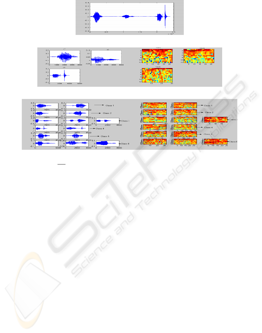
Figure 1: Discrete speech sound signal

Figure 2: Speech signals and their feature vectors

Figure 3: Training set and the training feature vectors

Thus, for each

nk ,1=

, the written word

corresponding to speech signal

is identified as

)(

. The transcript of the entire speech S results

as a concatenation of these labels.

Thus, the final result of our automatic speech

recognition process is the label

)(Sl

, computed as

follows:

)(...)()(

1 n

slslSl +

, (9)

where the meaning of the operator ‘+’ is the string

concatenation.

6 EXPERIMENTS

In this section we present some practical results of

our experiments. We have tested the described

recognition system for English language and

obtained many satisfactory results. We get a 80%

speech recognition rate using the proposed

approach. For space reasons we present a simple

test in this paper.

Thus, we consider a discrete vocal sound whose

speech has to be recognized. Its signal S is the one

represented in Figure 1. We perform a vocal

segmentation on S, using T = 0.01, and the three

speech signals,

321

,, sss

, represented in Figure 2,

are thus obtained.

For each

, a delta delta mel cepstral feature

vector

)(

is then computed. The feature

vectors are displayed as color images in Figure 2.

We use in this experiment a very small English

vocabulary, which is: {car, John, apple, help,

hurry, needs}. All the spoken words of S belong to

this vocabulary.

We consider three speakers for the third and

the last word, and only two speakers for each of

the others. Thus, the following training set is

obtained: {

,,,,,,,,, SSSSSSSSSS

S }. All these prototype signals are displayed

in Figure 3. The signals related to i

class are

represented on the row i.

Therefore, for these classes we obtain the

following labels: l(1) = ’car’, l(2) = ’John’, l(3) =

‘apple’, l(4) = ‘help’, l(5) = ‘hurry’ and l(6) =

’needs’. The training feature vectors

)(

, as

they result from the delta delta mel cepstral

analysis, are represented as color images in the

same figure.

We compute first the distances given by (7)

between the feature vectors displayed in Figure 2

and the training vectors displayed in Figure 3. For

DISCRETE SPEECH RECOGNITION USING A HAUSDORFF BASED METRIC - An automatic word-based speech

recognition approach

367

each

the mean distance to each class is then

computed. The obtained values are registered in

the next table.

Tab1e 1

1 2 3 4 5 6

)(

4.10 3.02 4.36 4.27 3.99 5.19

)(

6.41 4.24 5.46 5.79 6.59 3.01

)(

3.36 3.03 2.91 2.76 3.53 4.47

As it results from Table 1, the minimum mean

distance from

)(

to a training feature vector

set is 3.02. This value corresponds to the second

class, therefore

must be inserted in that class

and

'')2()(

Johnlsl ==

From the table row related to

)(

it results

that the minimum mean distance value is 3.01 and

it is related to the sixth class. Therefore, we get

'')6()(

needslsl ==

. For the third feature

vector,

)(

, the minimum mean distance is

2.76 and it is related to the fourth class. Thus,

'')4()(

helplsl ==

The final speech recognition result, being the

label of vocal signal S, is obtained as

)()()()(

321

slslslSl ++=

. This means that the

initial vocal sound speech transcript is

' ')( helpneedsJohnSl =

7 CONCLUSIONS

We have described a model for an automatic

speaker-independent word-based discrete speech

recognition system. The main novelty brought by

this work is a nonlinear metric which works

properly in discriminating between different sized

speech feature vectors.

There exist Hausdorff-based metrics utilized in

image processing domain. We have created such a

distance which works in the speech recognition

field.

Also, we have tested our method and obtained

good results. In our experiments low-size

vocabularies were used. Our idea is to extend such

a vocabulary over time, adding more and more

words, until it reaches a considerable size.

Obviously, the Hausdorff-based distance we

have provided will work properly with other types

of speech recognition approaches, which were

mentioned by us in the introduction. Thus, our

future research will focus on the continuous speech

recognition and the phoneme-based speech

recognition. In both cases we want to keep using

this nonlinear metric in the feature classification

stage.

REFERENCES

Rabiner, L., Juang, B. H., 1993. Fundamentals of Speech

Recognition. Prentice Hall Signal Processing Series.

Prentice Hall, Englewood Cliffs, New Jersey 07632,

A. V. Oppenheim, Series Editor.

Rabiner, L., Schafer, R., 1978. Digital Processing of

Speech Signals. Prentice Hall Signal Processing

Series. Prentice Hall, Englewood Cliffs, NJ.

Minh N. Do, 2000. An Automatic Speaker Recognition

System. Digital Signal Processing Mini-Project.

Audio Visual Communications Laboratory, Swiss

Federal Institute of Technology, Lausanne.

Furui, S, 1986. Speaker-independent isolated word

recognition using dynamic features of the speech

spectrum. IEEE Transactions on Acoustic Speech

and Signal Processing. Vol ASSP-34, No.1, 52-59.

Logan B., 2000. Mel Frequency Cepstral Coefficients

for Music Modelling. In Proc Int. Symposium on

Music Information Retrieval (ISIMIR). Plymouth,

MA.

Gregoire, N., Bouillot, M., 1998. Hausdorff distance

between convex polygons. Web project for the

course CS 507 Computational Geometry, McGill

University.

Duda, R., Hart, P., Stork, D., G., 2000. Pattern

Classification. John Wiley & Sons.

ICETE 2004 - WIRELESS COMMUNICATION SYSTEMS AND NETWORKS

368