
PERFORMANCE ANALYSIS OF A SPLIT-LAYER MULTICAST
MECHANISM WITH H.26L VIDEO CODING SCHEME
Naveen K Chilamkurti
Ben Soh
Sri Vijaya Gutala
Applied Computing Research Institute
La Trobe University, Melbourne
Victoria, Australia-3086
Abstract Support for video transmission is rapidly becoming a common requirement. Video coding schemes such as
H.26L are combined with multilayer multicast protocols such as SPLIT to improve the quality of video
received at the receiver. In this paper, we built a simulation system using a modified version of JVT (Joint
Video Team) encoding / decoding software package and Network Simulator NS-2, to evaluate H.26L video
transmission over SPLIT. System performance was observed in terms of Loss Ratio, Video Jitter,
throughput and PSNR for quality of the transmitted video.
1 INTRODUCTION
In an era of proliferating multimedia applications,
support for video transmission is rapidly becoming a
basic requirement of network architectures.
Furthermore, since most video applications (e.g.,
teleconferencing, television broadcast, and video
surveillance) are inherently multicast in nature,
support for point-to-point video communication is
not sufficient. Unfortunately, multicast video
transport is severely complicated by variation in the
amount of bandwidth available throughout the
network (Xue, 1999).
A scalable solution to the problem of available
bandwidth variation is to use multi-layered video. A
multi-layered video encoder encodes raw video data
into one or more streams, or layers, of differing
priority. However, multi-layered video is not by
itself sufficient to provide ideal network bandwidth
utilization or video quality (Mccanne, 1996).
The SPLIT-Layer Video Multicast Protocol is a
receiver based rate adaptation scheme solely
intended for single source video transmission
(Chilamkurti, 2003). By ‘splitting’ each encoded
video layer into two streams SPLIT is able to
provide an end receiver with the most relevant video
data so that the error concealment techniques can
better reproduce the encoded video under lossy
conditions.
In this paper, we simulate the transmission of H.26L
encoded streams over SPLIT. H.26L is the newest
and most efficient video coding scheme developed
by the International Telecommunication Union
(ITU) (H.26L, 2003). It uses a number of tools that
allow it to deliver much more efficient video coding
in low bit-rate applications than any MPEG
standard.
2 H.26L – A VIDEO
COMPRESSION STANDARD
2.1 H.26L: Overview
The main objective behind the H.26L project is to
develop a high-performance video-coding standard
by adopting an approach where simple and
straightforward design using well-known building
blocks are used. The ITU-T Video Coding Experts
Group (VCEG) has initiated the work on the
standard in 1997. The emerging H.26L standard has
a number of features that distinguish it from existing
standards, while at the same time, sharing common
features with other existing standards (Greenbaun,
1999).
Some of the key features of H.26L are (1) Saves up
to 50% in bit rate savings (2) High quality video (3)
181
K. Chilamkurti N., Soh B. and Vijaya Gutala S. (2004).
PERFORMANCE ANALYSIS OF A SPLIT-LAYER MULTICAST MECHANISM WITH H.26L VIDEO CODING SCHEME.
In Proceedings of the First International Conference on E-Business and Telecommunication Networks, pages 181-186
DOI: 10.5220/0001385701810186
Copyright
c
SciTePress

Adaptation to delay constraints (4) Error Resilience
and (5) Network friendliness.
3 SPLIT-A RECEIVER-ORIENTED
VIDEO MULTICAST
PROTOCOL
3.1 Overview
There are many receiver based rate adaptation
protocols capable of providing scalable rate
adaptation of multicast video traffic to
heterogeneous receivers. SPLIT-Layer Video
Multicast Protocol (SPLIT) however is specifically
designed to take advantage of existing encoding
techniques to provide the end user with an increased
perceived video quality.
SPLIT works by having the source S encode n (n >
1) video layers (V) where V1 is the base layer and
every additional layer V2,..,Vn is enhancement
layers. Each layer is then ‘split’ into two streams
VnHP and VnLP where VnLP contains aprox. 1/n-1
of Vn. VnHP and VnLP are then transmitted to
separate multicast address at a high and low priority
respectively (IPv6 Priority field). Each destination
wishing to join a video session will begin by
subscribing to the base layer (V1HP and V1LP) after
t time intervals if there is no congestion the receiver
will add V2HP and V2LP and again wait t time
intervals and if there is still no congestion the
process will be repeated until either the receiver has
joined all 2n multicast sessions or congestion is
detected.If destination D has subscribed to m video
layers (that is V1HP and V1LP to VmHP and
VmLP) detects congestion (determined by packet
loss rate) and has not recently received a join
experiment message the destination will drop VmLP
and begin using the hybrid loss concealment to
estimate the data lost from VmLP if packet loss rate
is still to high the layer containing Vm-1LP will be
dropped and estimated and so on. If after dropping
layer V1LP congestion remains a problem layer
VmHP is dropped, layer VmLP and Vm-1LP remain
dropped and layers V1LP to Vm-2LP are reinstated.
The sequence is repeated with m now equal to m-1
until acceptable packet loss is obtained or only layer
V1HP remains.
If receiver R1 is currently subscribed to layer n and
receiver R2 (who shares a bottleneck point with R1)
is subscribed to layer n + 1 and both suffer
congestion from the same cause (i.e. at the shared
bottleneck) and receiver R1 drops layer n this will
have no effect on the congestion unless R2 drops
layers n + 1 and n. Therefore the acceptable length
of time for a receiver to be congested (i.e. wait to
drop a layer) will be a function of the number of
layers the receiver is currently subscribed to. After
dropping a layer a receiver will send a drop layer
message stating the layer that has been dropped so
that receivers in the area receiving a lower layer can
hold off from dropping a lower layer until
surrounding receivers drop layers higher than the
one the receiver is currently subscribed to. After a
successful layer drop (i.e. no more congestion) the
receiver will send an end congestion message to
surrounding receivers so that any lower layer
receiver that is still congested can proceed to drop
appropriate layers. Any receiver that feels it has
been in a state of congestion for too long a period
can drop the appropriate layers.
Before beginning a join experiment a receiver sends
a join experiment notification message addressed to
the base layer in the local area (determined by IP
multicast scope) with IPv6 priority set to 7 (internet
control traffic) (Hinden, 1995). If the experiment
fails (causes congestion) the layer is dropped and
any other receivers in the area that were affected by
the congestion do not drop layers until some time
after the experiment. If congestion remains this may
be improved by a layer dropped message. If the
experiment is a success a join success message is
sent so that any receiver who suffered congestion
shortly after receiving a join message can begin to
drop layers as the congestion was caused by an
external event. (i.e. not the join experiment)
4 EXPERIMENTATION SETUP
4.1 Overview
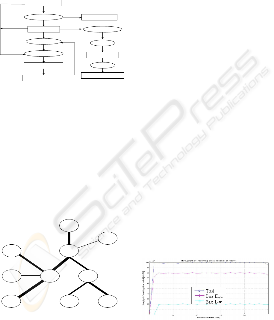
In order to evaluate the video transmission over
SPLIT, we set up the simulation system, which is
illustrated in Figure 1 to gather data for our analysis.
The data and process point of views of the
simulation set-up is demonstrated in the Figure 2.
Figure 1: Simulation system block Diagram
Video Source PSNR Measure
Decode
Video
JM Decode
r
JM Encode
r
NS-2
RTP Paketize
r
Loss Profi
t
ICETE 2004 - WIRELESS COMMUNICATION SYSTEMS AND NETWORKS
182
We first feed a sample video source (Foreman. CIF),
a raw video sequence in QCIF (Quarter Common
Image Format) [4:2:0] format to the encoder.
Figure 2: Data and Control Flow of the Simulation System
5 SIMULATING SPLIT
SPLIT is simulated using (NS-2, 1999) and all the
necessary information to configure and control the
simulation is stored in a file using Otcl script. The
simulation objects are instantiated with the script,
and immediately mirrored in the compiled hierarchy.
The input script defines the topology, builds the
agents, sets the trace files and sets the start times for
the initial events in the simulation.
5.1 Topology
The following network topology was defined to run
the simulations.
Figure 3: Topology of the Simulation
The sample topology consists of a single source,
three routers and six destination nodes. Each node is
connected at a different bandwidth ranging from
1Mbs to 10Mbs. The source will be transmitting a
scaled five layer stream, consisting of 1Mbs per
layer with a packet size of 1Kb, the SPLIT source
will ‘split’ each layer into a high and low priority
streams at a ratio of 4:1. (I.e. 80% for high priority
and 20% for low priority streams). This will be
simulated in NS-2 as a ten (five high and five low
priority) constant bit rate (cbr) flows. We use TCP
as the back ground traffic. We generate a video trace
and attach it to the source. At t= 0.01 Sec source
transmits the CBR data stream to all the receivers.
At t=1 Seconds both TCP and trace data applications
begin to transmit frames with the interval of 10ms.
5.2 Routing and Queuing
A dense mode of multicast routing algorithm is used
during simulations with the prune time-out set to 30
seconds. This was to ensure that the operation of
SPLIT could be fully examined without any
interference from the underlying routing protocol.
Each router was implemented using the RED
(Random Early Detection) (Floyd, 1993) queue so
that optimal transmission rates of the base layers
could be achieved through RED queue and its
priority stream.
6 EXPERIMENTATION RESULTS
AND ANALYSIS
To evaluate the visual quality of the video, the
simulations are run under two different scenarios.
The first scenario (UDP-H26L) provides the
baseline for comparing our results of visual quality.
The application simply hands down each video
frame to the UDP layer. In the second scenario, the
frames are handed to the SPLIT Source (SPLIT-
H26L).
6.1 Throughput at Receivers:
Figure 4: Throughput of Receiving bits at Receiver1
10Mbs
1Mbs
4Mbs
2.5Mbs
3.5Mbs
2.5Mbs
2.5Mbs
5Mbs
5Mbs
Source
Dest. 1
Dest. 2 Dest. 3
Dest. 4
Dest. 5
Dest. 6 R1
R3 R2
AWK
Foreman.YUV
Foreman.qcif
JM Encoder
Foreman.26L
RTPDump
JM Decoder
Decoded Video
PSNR Result
Trace_Gen
NS-2
Output.tr
Loss Profile
PERFORMANCE ANALYSIS OF A SPLIT-LAYER MULTICAST MECHANISM WITH H.26L VIDEO CODING
SCHEME
183
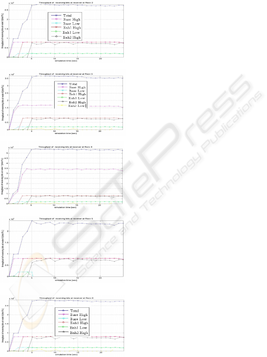
Figure 5: Throughput of Receiving bits at Receiver2
Figure 6: Throughput of Receiving bits at Receiver3
Figure 7: Throughput of Receiving bits at Receiver4
Figure 8: Throughput of Receiving bits at Receiver5
Figure 9: Throughput of Receiving bits at Receiver6
Discussion:
Throughput is defined as the maximum rate at which
the switch can forward packets without packet loss.
Figures 4, 5, 6, 7, 8, and 9 represent throughput at
the receivers.
In this experiment Receiver 1 is connected to the
source at a bottleneck speed of 1Mbs.The available
bandwidth was fully utilized by SPLIT protocol and
Receiver1 being able to subscribe only the base
layer. This occurred because the available bandwidth
was not sufficient enough to enable the receiver to
subscribe to the high priority streams of both the
base and first enhancement layer.
The second set of results was taken from Receiver 2,
which is connected at a bottleneck speed of 2.5Mbs
to the source. In this experiment SPLIT was able to
fully and effectively utilise the available bandwidth
and was able to subscribe to the available video
layers.
The results shown in Figure 6 are taken from
Receiver 3, which is connected to the source at a
bottleneck speed of 3.5Mbs. In this instance the
SPLIT receiver was able to subscribe to three high
priority streams as well as the three low priority
streams. By sacrificing portions of each
enhancement layer with the view that packet loss
concealment mechanisms would be able to
reproduce the missing data SPLIT was able to
receive an extra enhancement layer.
Receiver 4 is connected to the source at a speed of
5Mbs, which is clearly sufficient to receive the five
1Mbs video layers being transmitted by the source.
As expected, Figure 7 shows that both the SPLIT
receivers had no problems in receiving the five
layers.
Receiver 5 was connected to the source at a
bottleneck speed of 2.5Mbs. As shown in Figure 8
the SPLIT receiver was able to subscribe to both the
high and low priority streams of the base layer as
well as the high priority streams of the first two
enhancement layers.
In this final experiment, Receiver 6 was connected
to the source at a speed of 2.5Mbps. As shown in
Figure 9 the SPLIT receiver was able to subscribe to
both the high and low priority streams of the base
layer as well as the high priority streams of the first
two enhancement layers.
The overall performance of SPLIT was quite good.
It was able to subscribe to all the available layers
and this leads to the increase in throughput at the
receiver. By being able to make a more effective use
ICETE 2004 - WIRELESS COMMUNICATION SYSTEMS AND NETWORKS
184
of the available bandwidth the SPLIT mechanism
ensures better video quality.
6.2 Loss Ratio
Loss ratio for a particular flow I is defined to be:
Loss Ratio = Number of packets dropped in flow I
Total packets received in flow
In this experiment, there were five layers of high
priority and low priority stream. The loss ratio is
computed for each flow from the trace file obtained
after the simulation and tabulated as follows:
Table 1: Loss Ratio in High Priority Layers
Number
of packets
received
Number
of
packets
dropped
Loss Ratio
Base High
Layer
67419 10 0.014832
Enhancement
High Layer1
55072 18 0.032684
Enhancement
High Layer2
50665 94 0.185532
Enhancement
High Layer3
37981 243 0.639793
The number of packets dropped was very low
compared to the number of packets received in all
the high priority layers. The mean loss ratio across
all the high priority layers subscribed is found to be
0.0021821025.
Loss Ratio in the lower priority layers:
Table 2: Loss Ratio in Low Priority Layers
Number
of packets
received
Number
of
packets
dropped
Loss Ratio
Base Low
Layer
14379 31 0.215592
Enhancement
Low Layer1
2625 124 4.723
Enhancement
Low Layer2
236 146 61.8644
Enhancement
Low Layer3
207 154 74.3961
The mean loss ratio in low priority layers is found to
be 0.240133 or 24%. But in SPLIT mechanism if a
destination D has subscribed to m video layers (that
is V1HP and V1LP to VmHP and VmLP) and
detects congestion then the destination will drop
VmLP. If packet loss rate is still too high then layer-
containing Vm-1LP will be dropped and so on.
Hence the loss rate in lower priority layers is found
to be high.
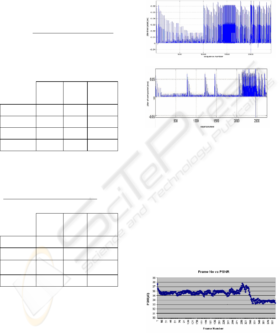
6.3 Video Packet Jitter:
Figure 10: Packet Jitter for video flow – UDP-H26L
Figure 11: Packet Jitter for video flow – SPLIT-H26L
Discussion:
Figure 10 and Figure 11 depict the video packet
jitters. The delay jitter values are taken for video
over UDP and SPLIT at Dest4. Packet jitter
experienced by UDP-H26L is more than SPLIT.
While in Video over SPLIT the jitter values were
ranging from 0.1 to 0.2. The reason for increase in
jitter for the first scheme is that UDP bursty nature
induces more jitter to the other competing flows.
Thus video application based on SPLIT will require
low play out buffers to absorb jitter than applications
based on UDP. Hence we can say from the results
obtained the SPLIT rate adaptation scheme helps in
reducing jitter effects.
6.4 Quality Measure: PSNR (Peak
Signal to Noise Ratio)
Figure 12: PSNR of UDP-H26L
PERFORMANCE ANALYSIS OF A SPLIT-LAYER MULTICAST MECHANISM WITH H.26L VIDEO CODING
SCHEME
185
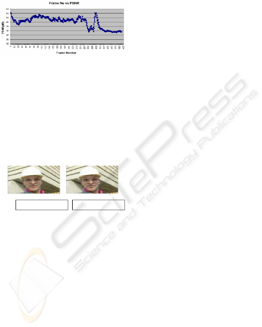
Figure 13: PSNR of SPLIT-H26L
Discussion:
PSNR values are compared by UDP-H26L and
SPLIT-H26L schemes by streaming a QCIF foreman
sequence encoded with H26L. Figures 12 and 13
compares the PSNR values of the foreman sequence
encoded using the H26L codec with and without
SPLIT protocol. Figure 12 corresponds to the
simulations with UDP source, 5Mbps bottleneck
bandwidth. In this case, for the foreman sequence,
an average PSNR of 34.44 was obtained. The
average PSNR obtained was 37.25. We can see from
the graphs that under similar network conditions, the
source with SPLIT gave better PSNR results. On
average a gain of 3dB is found.
Figure 14: Foreman sequence used in simulations
Besides the subjective performance of the two
schemes, snapshots of the decoded Foreman
sequence are shown in Figure 14. The visual quality
of the video transmitted with SPLIT is found to be
better.
7 CONCLUSIONS AND FURTHER
RESEARCH
In this paper, we built a simulation system using
Network Simulator NS-2, to evaluate H.26L video
transmission over SPLIT. System performance was
observed in terms of Loss Ratio, Video Jitter,
throughput and PSNR for quality of the transmitted
video.
It was observed that, in the proposed system, video
layers of high priority do not experience much loss,
because the SPLIT mechanism makes all lost
packets concentrated in video layers of lower
priority.
To evaluate the visual quality of the video sequence,
two scenarios were considered. In the first case,
video traffic was transferred from source to the
destination using UDP. The simulation results
showed a low jitter value and a high quality image at
the decoder under congestion by being able to
subscribe extra enhancement video layers, whilst
keeping packet loss under a threshold.
Our future research is to establish a mapping
between the packet level loss pattern and loss pattern
on a video level. This is of utmost importance since
it will enable relating the end-user perception to the
packet level loss, which might provide a reference
basis for effective error correction or error
concealment techniques at the end hosts.
REFERENCES
Xue Li, Mostafa H. Ammar, Sanjoy Paul, 1999.Video
Multicast over the Internet. IEEE Network Magazine.
Steven McCanne, Van Jacobson, Martin Vetterli.1996.
Reciever-driven Layerd Multicast. In proceedings of
ACM SIGCOM.
N.Chilamkurti, B.Soh, B.Simmon.2003. SPLIT: A New
Receiver-oriented Video Multicast Protocol. In
proceedings of IEEE NCA. IEEE press.
Emerging H.26L Standard – Overview and TMS320O64X
,Implementation.UB Video Inc. , URL
http://www.ubvideo.com.
G.S.Greenbaun.1999. Remarks on the H.26L project:
streaming video requirements for next generation
video compression standards”, ITU-T SG16/Q1.5.
R.Hinden, S.Deering. 1995. RFC 1884 IP version 6
Addressing Architecture. IEEE draft.
Ns-2 network simulator, URL
http://www.isi.edu/nsnam/ns/
S.Floyd and V. Jacobson. 1993. Random early detection
gateways for congestion avoidance. IEEE/ACM
Transactions on networking. IEEE Press.
Without SPLIT With SPLIT
ICETE 2004 - WIRELESS COMMUNICATION SYSTEMS AND NETWORKS
186
