
ONLINE SMOOTHING OF VBR VIDEO STREAMS IN SYSTEMS
WITH VARIABLE AVAILABLE BANDWIDTH
Pietro Camarda, Antonio De Gioia, Domenico Striccoli
Politecnico di Bari – Dip. di Elettrotecnica ed Elettronica, Via E. Orabona, 4 – 70125 Bari (Italy)
Keywords: Video Distribution, VBR traffic, Online Smoothing, Available Bandwidth
Abstract: Compressed multimedia transmission is assuming a growing importance in the
telecommunication world. However, the high data rate variability of compressed video over
multiple time scales makes an efficient bandwidth resource utilization difficult to obtain.
Smoothing techniques is one of the approaches exploited to face this problem. Various
smoothing algorithms have been proposed, that reduce the peak rate and high rate variability of
video streams by efficiently prefetching video data to be transmitted over the network. However,
all previous algorithms consider a constant available bandwidth. Such a constraint can be hardly
verified in modern telecommunication networks. In this paper a novel online smoothing
algorithm is proposed, that performs data scheduling by taking into account the residual available
bandwidth, and at the same time minimizing rate variability changes. This algorithm can be fully
exploited for online smoothing of video applications that want to tolerate very short playback
delays. Numerical results show that the proposed algorithm is very effective for online smoothing
purposes in a link sharing environment.
1 INTRODUCTION
The increasing computational capacity of modern
computers together with the sustained growth of
telecommunication networks bandwidth allow
multimedia streaming through bursty Variable Bit
Rate (VBR) stream transmission. As it can be seen
from Figure 1, the VBR source behavior makes the
optimization of network utilization more difficult
while providing at the same time Quality of Service
(QoS) guarantees, i.e., low delays and jitters, low
data losses, and so on (Kurose and Ross, 2000)
(Zhang et al., 1997).
To reduce the total amount of bandwidth
assigned to video streams, work-ahead smoothing
techniques can be exploited (Salehi et al., 1998)
(Feng and Rexford, 1997). These techniques are
based on the reduction of the peak rate and the bit
rate variability of network streams; they consist in
transmitting, ahead of playback time, pieces of the
same film with a constant bit rate that varies from
piece to piece according to a scheduling algorithm
that smoothes the bursty behaviour of video streams.
On the transmission side a buffer regularizes data
transmission, while on the receiving side the frames
are temporarily stored in a client buffer and
extracted during the decoding process. Obviously,
the bit rate must be chosen appropriately in order
to avoid buffer overflow and underflow, ensuring a
continuous playback at the client side. The client
smoothing buffer size determines number and
duration of the Constant Bit Rate (CBR) pieces that
characterize the smoothed video stream. An increase
of the smoothing buffer size generally produces a
smaller number of bandwidth changes among CBR
segments and a peak rate and rate variability
reduction of smoothed video streams (Zhang et al.,
1997) (Salehi et al., 1998).
As described in (Feng and Rexford, 1997), a
VBR video stream is composed by N video frames,
each of them of size
i
d bytes
(
. On the
server side, the stream data enter a buffer whose
capacity is bytes, and the buffer output gives the
smoothed video stream data. At the client side, the
smoothed video data enter the buffer and the original
unsmoothed video frame sequence leaves the buffer.
Let us now consider the client buffer model in the
discrete frame time, that is, the time interval in
)
Ni ≤≤1
b
th
k
369
Striccoli D., Camarda P. and De Gioia A. (2004).
ONLINE SMOOTHING OF VBR VIDEO STREAMS IN SYSTEMS WITH VARIABLE AVAILABLE BANDWIDTH.
In Proceedings of the First International Conference on E-Business and Telecommunication Networks, pages 369-374
DOI: 10.5220/0001388103690374
Copyright
c
SciTePress
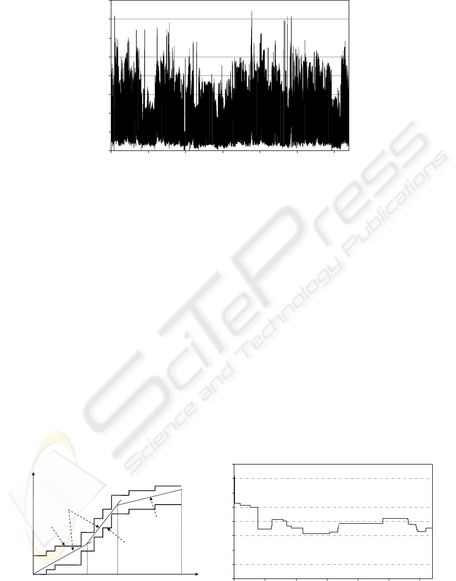
0
20
40
60
80
100
120
140
160
0 5000 10000 15000 20000 25000 30000
Frame number
Frame size (kbits)
Figure 1: 32.000 video frames of the “Simpson’s” cartoon, codified with the MPEG-1 algorithm.
which a video frame is transmitted. To guarantee
a feasible transmission, the cumulative amount of
data consumed by the client buffer at discrete time k:
∑
=
=
k
i
i
dkD
1
)(
(1)
should arrive quickly enough to avoid buffer
underflow At the same time, to avoid buffer
overflow, at time k the client buffer should not
receive more data than:
∑
=
+=
k
i
i
dbkB
1
)(
(2)
The cumulative smoothed data have to respect
the following bounds:
)()()(
1
kBiskD
k
i
≤≤
∑
=
(3)
where
represents the smoothed stream bit
rate in the discrete frame time i, while
are the cumulative smoothed data
arrived to the client buffer until frame time k. The
smoothed stream transmission plan will result in a
number of CBR segments, and the correspondent
stream evolution is given by a monotonically
increasing and piecewise-linear path that lies
between the
and curves, as can be
shown in Figure 2a. According to the definition
given in (Feng and Rexford, 1997), each CBR
segment defines a run that can be considered as a
frontier of possible starting points for the next run.
)(is
∑
=
=
k
i
iskS
1
)()(
)(kD
)(kB
As described in (Feng and Rexford, 1997),
different types of smoothing algorithms can be
implemented; all of them transform the highly bursty
video stream bit rate behaviour into a series of CBR
pieces. The scheduling algorithm regulates each of
the CBR bit rate values in such a way to respect the
buffer constraints
and . Now let us
examine more in detail some of the most common
smoothing algorithms proposed in literature.
)(kD
)(kB
The Critical Bandwidth Allocation (CBA)
algorithm minimizes the number of bandwidth
increases as follows. For bandwidth decreases, the
rate decrease starts in the earliest point in time, when
the previous run hits the lower bound curve. For
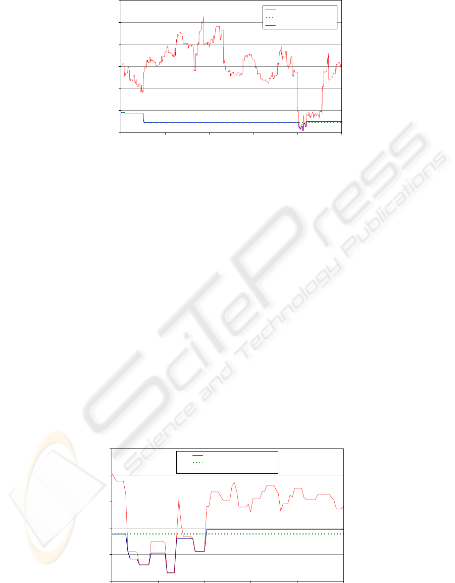
Frame size
[
b
y
tes
]
b
Time
(
frames
)
CBR segment
B
(
k
)
D(k)
Fr
o
nti
e
r
s
0
5
10
15
20
25
30
35
40
0 5000 10000 15000 20000 25000 30000
Frame number
Frame size (kbit)
Figure 2a: An example of smoothed video stream
transmission plan.
Figure 2b: The “Simpson’s” cartoon, MVBA
smoothed (buffer size 1024 kbytes).
ICETE 2004 - WIRELESS COMMUNICATION SYSTEMS AND NETWORKS
370

bandwidth increases, the starting point of the next
run is chosen in such a way that it extends as far as
possible. In this way, the transmission plan has the
smallest peak bandwidth requirement and the
minimum number of bandwidth increases (Feng and
Sechrest, 1995).
The Minimum Changes Bandwidth Allocation
(MCBA) algorithm minimizes both the number of
bandwidth increases and decreases by performing
the same research of the next run starting points
made in the CBA algorithm, for bandwidth
increases. This results in a transmission plan that
minimizes the number of bandwidth increases,
bandwidth decreases, and also the peak bandwidth
requirement (Feng et al., 1996).
The Minimum Variability Bandwidth Allocation
(MVBA) algorithm reduces the bandwidth change
variability by searching, for each CBR piece, the
earliest point in time in which a bandwidth increase
or decrease can happen, obviously respecting at the
same time the lower and upper constraints. The
corresponding transmission plan gradually performs
rate changes, assuring in this way the smallest
variability of rate changes, at the expense of a
greater number of CBR pieces if compared with
CBA and MCBA algorithms (Salehi et al., 1998)
(Feng and Rexford, 1997).
The Piecewise Constant Rate Transmission and
Transport (PCRTT) algorithm divides the video flow
into time intervals with fixed temporal dimension in
which the assigned bandwidth changes. The
transmission plan is obtained by creating a CBR
piece in each time interval; the bit rate is obtained by
connecting the extreme points of the lower bound
curve. The segment slope represents the bit rate of
the CBR piece. Finally, the segment is raised in such
a way to be included among the two bound curves,
avoiding buffer underflow (Feng and Rexford, 1997)
(McManus and Ross, 1996). An enhanced version of
the PCRTT algorithm, called e-PCRTT, can be
found in (Hadar and Cohen, 2001). It behaves like
the PCRTT algorithm, but it is capable to reach the
same transmission plans of the original PCRTT
algorithm with smaller smoothing buffers, or
alternatively, given the same buffer sizes, it reduces
the number of bandwidth changes. Furthermore, it
reduces also the playback delay if compared with the
PCRTT algorithm.
The choice of each of the mentioned algorithms
depends on what aspect of data transmission has to
be optimized among the peak rate, number,
variability and periodicity of bandwidth changes.
An example of the application of the smoothing
algorithm can be observed in Figure 2b.
All the mentioned smoothing techniques mainly
apply to stored video traffic, where all source video
data are a priori known and can be optimally
scheduled in an “off-line” manner. The optimality of
the offline algorithms derive from the a priori
knowledge of the entire video data to be scheduled.
Nevertheless, the algorithms can also be applied in
an “on-line” manner, in limited temporal windows.
In this case, smoothing algorithms generally have a
limited a priori knowledge of frame sizes in short
consecutive temporal observation windows, thus
reducing video burstiness in a smaller time scale
and with a less efficient transmission plans (Rexford
et al., 1997); nevertheless, they remain. effective to
reduce peak rate and rate variability in the temporal
window of interest. In this context of online video
smoothing the proposed algorithm can be introduced
and exploited.
2 THE ABSA SMOOTHING
ALGORITHM
In this section the Available Bandwidth Smoothing
Algorithm (ABSA) is proposed and implemented,
taking into account not only the parameters of the
smoothing algorithms proposed in literature, i.e.,
buffer size and unsmoothed data, but also the
available residual bandwidth, that fluctuates in time
due to the presence of other traffic running into the
network. The ABSA algorithm represents a
substantial novelty if compared with the other
classical smoothing algorithms already analyzed; it
can be efficiently exploited in an online smoothing
context. The a priori knowledge of available
bandwidth resources in the considered time window
is an important requirement; thus available
bandwidth necessary for implementing the stream
bandwidth plan, is supposed to be a priori known
through bandwidth estimation techniques.
Let us suppose to analyze the video data
transmission in a temporal window of length N
video frames., at the same time knowing the
temporal evolution of available bandwidth
in
the frame time k. The two bounds (1) and (2) change
as follows. First of all:
)(kw
)()( kwks
≤
,
Nk
≤
≤
0
that is
)1()()()()1()( −+≤⇒
≤
−
−
kSkwkSkwkSkS
,(4)
Furthermore, according to (3), it has to be:
)()( kBkS
≤
Thus, calling:
[
]
)1()(),(min)(
,,
−+
=
kSkwkBkU
kUkS
wBS
it follows:
)()(
,, wBS
,
Nk
≤
≤
0
≤
It has to be pointed out that the bound
,,
U
wB
depends on the available bandwidth
, the
transmission plan and the curve..
)(k
w
S
)(kS
)(kB
ONLINE SMOOTHING OF VBR VIDEO STREAMS IN SYSTEMS WITH VARIABLE AVAILABLE BANDWIDTH
371
0
20
40
60
80
100
120
0 200 400 600 800 1000
Frame number
Bandwidth (kbit/frame)
ABSA algorithm
MVBA algorithm
Available bandwidth
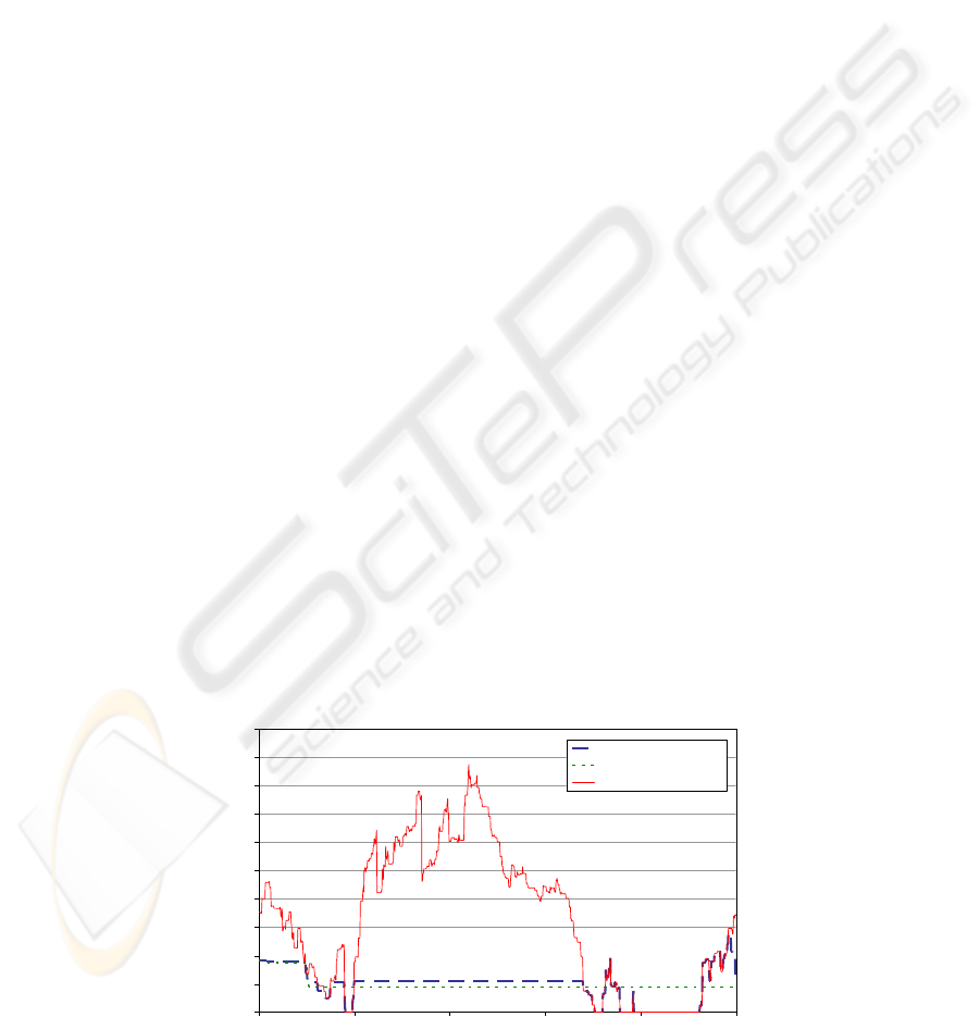
Figure 3: A comparison between the ABSA and MVBA smoothing algorithms. The window size is 1000 video frames.
Similarly, exploiting again(3) and (4):
; .
)()()1( kwkSkS −≥− )()( kDkS ≥
Defining the function:
[
)1()1(),(max)(
,,
+−+= kwkSkDkL
wDS
]
with the obvious further condition:
)()(
,,
NDNL
wDS
=
It is satisfied that:
)()(
,,
kLkS
wDS
≥
,
Nk
≤
≤0
We have:
)()()(
,,,,
kUkSkL
wBSwDS
≤≤
(5)
Nk ≤≤0
The main problem of the
and
calculation is that they depend on the scheduled data
in the previous and following steps. The dependence
of
and from the scheduled data
is thus eliminated by introducing the functions
)(
,,
kL
wDS
)(
,,
kU
wBS
)(
,,
kL
wDS
)(
,,
kU
wBS
)(kS
)]()1('),(min[)('
,,
kwkUkBkU
wBwB
+−=
,
with the initial condition
, and
)0()0('
,
BU
wB
=
)]1()1('),(max[)('
,,
+
−+= kwkLkDkL
wDwD
with the initial condition
.
)()('
,
NDNL
wD
=
It can be demonstrated that, if
is a feasible
transmission (that is,
),then:
)(kS
)()()(
,,,,
kUkSkL
wBSwDS
≤≤
k∀
wBSwB
UU
,,,
' ≥
; (6)
wDSwD
LL
,,,
' ≤
Proof:
It is valid that
)0()0(')0(
,,,
BUU
wBwBS
=
=
Let us proceed by induction and suppose that (6)
is valid in k. We have to show that (6) is valid in
k+1. It will be:
≥
+
+
+
=
+
)]1()('),1(min[)1('
,,
kwkUkBkU
wBwB
≥+
+
+
≥ )]1()(),1(min[
,,
kwkUkB
wBS
)1()]1()(),1(min[
,,
+
=+
+
+
≥ kUkwkSkB
wBS
.
This demonstrates the first of (6). Similarly, the
second of (6) can easily be demonstrated.
Thus is valid that:
wBwD
USL
,,
''
≤
≤
(7)
with the further advantage that
wD
and
are two bounds for
, that are independent from
itself. For this reason, a first approach to find the
transmission plan
is to apply the MVBA
smoothing algorithm as described in (Salehi at al.,
1998) with the two boundaries expressed by the
wD
and curves. If a frame time is found in
which
wBwD
, the corresponding transmission
plan
will not be feasible and the smoothing
algorithm can not be applied due to the strong
L
,
'
wB
U
,
'
S S
S
L
,
'
wB
U
,
'
UL
,,
'' >
S
0
5
10
15
20
25
800 820 840 860 880 900
Frame number
Bandwidth (kbit/frame)
ABSA algorithm
MVBA algorithm
Available bandwidth
Fi
g
ure 4: ABSA and MVBA in the critical time zone, where the available bandwidth consistentl
y
lowers.
ICETE 2004 - WIRELESS COMMUNICATION SYSTEMS AND NETWORKS
372
limitation in available bandwidth.
Let us now suppose to have verified (7) and
consequently (5), where the transmission plan
has been obtained through the optimal MVBA
smoothing algorithm (Salehi at al., 1998). In this
case, the ABSA smoothing algorithm behaves
exactly like the MVBA optimal smoothing
algorithm. If instead (5) is not effectively verified
for each
after have calculated (7) the
ABSA algorithm adjusts the CBR segment slopes of
(and consequently the constraint curves
wDS ,,
and
wBS
U
,,
) in such a way that (5) is verified for
each k, at the same time maintaining the scheduling
the closest possible to the optimal MVBA
smoothing algorithm curve. To better explain this
concept, let us suppose to have verified (5) for
1
, and that in frame time
1
, (5) is not
verified. The ABSA algorithm progressively
increases, in an iterative way, the value of
1
since it verifies (5) in
1
)(kS
Nk ≤≤0
S
L
S
10 −≤ k≤ k
kS
k
)(
kk
=
. This final step will
surely be reached, since if we assign:
)(')(
1,1 wB
it can be easily verified that:
kUkS =
,
kLkUkU
wB
w
≤≤
)(kS
in
k ,1+
. (8)
)()(')(
1'1,1,,'
,
UwBwBU
BwB
After the calculation of
1
, the optimal
MVBA algorithm is applied again starting from
and ending at and then verifying (5)
]
N
1
through the same procedure previously
illustrated.
,,
(9)
1
kk = Nk =
[
3 NUMERICAL RESULTS
In this section some numerical results are provided,
to testify the effectiveness of the proposed
algorithm. Different simulation scenarios have been
considered, and the algorithm performance has been
tested for different video stream types, different
smoothing buffers and temporal observation window
sizes. The available bandwidth information, in this
specific case, has been derived in the hypothesis that
other smoothed video streams form the background
traffic, consisting of 12 MVBA-smoothed video
streams. Flow aggregation has been performed
randomly choosing the video stream starting points
and deriving the total bandwidth occupied by stream
aggregation simply by adding the number of bits
contained in each video streams frame, in each
discrete time unit given by a frame transmission
time. In this case, the so obtained bandwidth is
expressed in bit/frame. Supposed a channel capacity
C, the available bandwidth has been derived simply
subtracting the bandwidth exploited by stream
aggregation previously calculated to C, in each
frame time and supposing to know in advance all the
flow aggregation information in each frame time.
Established the temporal observation window
size (in frame number), the ABSA algorithm is then
applied. A first comparison among the ABSA and
MVBA smoothing techniques is illustrated in Figure
3. A temporal window of size 1000 video frame has
been chosen; taking into account a constant frame
rate of 25 frames/s, the temporal window size is 40
s. In this window a piece of the “James Bond:
Goldfinger” video stream, MPEG-1 codified, has
been smoothed with both the MVBA and the ABSA
smoothing algorithms, highlighting the main
differences between them. From Figure 3 it can be
noted that there is a strong available bandwidth
reduction, beginning from the 807
th
frame until the
843
th
frame, due to high bandwidth requirements by
flow aggregation already present in the network link.
During this period the ABSA smoothing algorithm,
represented through a continuous blue line, follows
perfectly the available bandwidth curve (depicted as
a continuous red line), while the MVBA algorithm
crosses the red line, testifying a frame loss that
occurs until the available bandwidth curve raises
again. This important particular can be better
0
10
20
30
40
50
60
70
80
90
100
0 200 400 600 800 1000
Frame number
Bandwidth (kbit/frame)
ABSA algorithm
MVBA algorithm
Available bandwidth
Figure 5: The ABSA and MVBA smoothing algorithms, for stronger available bandwidth reduction.
ONLINE SMOOTHING OF VBR VIDEO STREAMS IN SYSTEMS WITH VARIABLE AVAILABLE BANDWIDTH
373

appreciated by observing Figure 4, in which an
enlargement of the critical time interval, in which
the available bandwidth falls down quickly, is
reported.
As can be noted from Figure 4, the ABSA
algorithm transmission plan raises again after have
passed the strong bandwidth reduction zone (after
the 843
th
video frame), continuing with a long CBR
segment, according with the ABSA algorithm
purpose of performing the MVBA smoothing
technique whenever possible. Anyway, in the last
time period the bandwidth level reached by the
ABSA algorithm is higher than the corresponding
MBA offline smoothing transmission plan. This is
obvious, since the ABSA algorithm has to
compensate in some way the lower bit rates
scheduled during the strong bandwidth reduction
zone. In Figure 5 another comparison among the two
proposed algorithms is depicted, in more critical
available bandwidth conditions.
In Figure 5 two “critical zones” , in which the
available bandwidth strongly falls down, can be
observed; the first is clearly visible on the left of the
figure, beginning in the 105
th
video frame and
ending at the 200
th
video frame. In this first critical
zone, the available bandwidth is sometimes null. The
second critical zone starts from the 680
th
video frame
and ends at the 930
th
video frame. In this second
critical zone a major lacking of available bandwidth
can be noted, and the time interval in which
available bandwidth reaches zero is longer. The
utilization of the MVBA algorithm would result in
very consistent frame losses, while the ABSA
algorithm produces no losses all the time, perfectly
following the available bandwidth curve. In the
second critical zone on the right, it can be noted that
the ABSA algorithm continues following the
available bandwidth curve long after the critical
zone is finished, since there is no other way to
recover from the heavy resource lacking previously
occurred. It can be easily verified that the ABSA
algorithm behaviour appears very effective also if
applied to other types of films, with different
smoothing buffer and/or temporal window sizes.
4 CONCLUSIONS AND FUTURE
WORK
In this paper, a novel smoothing algorithm, called
ABSA algorithm, has been developed and analyzed.
The main novelty of this algorithm is that it is able
to take into account residual available bandwidth
fluctuations, trying to adapt the smoothing
transmission plan to available bandwidth resources,
at the same time trying to keep, whenever possible,
the main advantages of the MVBA smoothing
algorithm. Numerical results show that the ABSA
algorithm performs better than the MVBA algorithm
in all cases of reduced available bandwidth
resources, avoiding packet losses also in critical free
bandwidth conditions. This makes the ABSA
algorithm suitable for a more efficient packet
transmission planning. Nevertheless, some other
aspects of the ABSA algorithm have to be
investigated, like more efficient ways to modify the
ABSA transmission plan to minimize losses, or the
ABSA algorithm enhancement for a flow
aggregation. This last aspect would be of a great use
to avoid scalability problems, at the same time
optimizing bandwidth resource saving.
REFERENCES
Kurose, J. & Ross, K., 2000. Computer Networking: A
Top-Down Approach Featuring the Internet. Addison
Wesley Longman.
Zhang, Z.-L., Kurose, J., Salehi, J. D. & Towsley, D.,
1997. Smoothing, Statistical Multiplexing and Call
Admission Control for Stored Video. IEEE Journal on
Selected Areas in Communications, 15(6), 1148-1166.
Salehi, J.D., Zhang, Z.-L., Kurose, J. & Towsley, D.,
1998. Supporting Stored Video: Reducing Rate
Variability and End-to-End Resource Requirements
Through Optimal Smoothing. IEEE/ACM
Transactions On Networking, 6(4), 397-410.
Feng, W.-C. & Rexford, J., 1997. A Comparison of
Bandwidth Smoothing Techniques for the
Transmission of Prerecorded Compressed Video. In
IEEE INFOCOM.
Feng, W. & Sechrest, S., 1995. Critical Bandwidth
Allocation for Delivery of Compressed Video.
Computer Communication, 18, 709-717.
Feng, W., Jahanian, F. & Sechrest, S., 1996. Optimal
Buffering for the Delivery of Compressed Prerecorded
Video. In ACM SIGMETRICS.
McManus, J.M. & Ross, K.W., 1996. Video on Demand
over ATM: Constant-rate Transmission and Transport.
IEEE Journal on Selected Areas in Communications,
4(6), 1087-1098.
Hadar, O. & Cohen, R., 2001. PCRTT Enhancement for
Off-Line Video Smoothing. Journal of Real-Time
Imaging, 7(3), 301-314.
Rexford, J., Sen, S., Dey, J., Feng, W., Kurose, J.,
Stankovic, J. & Towsley, D., 1997. Online Smoothing
of Live Variable-Bit-Rate Video. In 7th Workshop
Network and Op. Systems Support for Digital Audio
and Video.
ICETE 2004 - WIRELESS COMMUNICATION SYSTEMS AND NETWORKS
374
