
INDOOR PROPAGATION MODELS AND RADIO PLANNING
FOR WLANS
Rui Lopes, Paulo Freixo e António Serrador
ISEL – Instituto Superior de Engenharia de Lisboa, Rua Conselheiro Emídio Navarro No.1, 1950-062 Lisboa, Portugal.
Keywords: WLAN, Indoor Propagation Models, 2
.4GHz Measurements, Planning
Abstract: WLANs are nowadays at the top of the mass market networks technologies. They are essentially
implemented indoors, where the traditional planning tools are not yet focused. In spite of the concern to
improve the radio planning quality, the existing propagation models can still be sharpened for better
outcomes, mainly in large buildings. A new propagation model is proposed and evaluated with
measurements at 2.4GHz and also a planning tool is presented, with the ability to execute coverage and
capacity analysis on indoor multi-floors environments. This model adapts itself to multiple indoor scenarios
following the performed measurements
1 INTRODUCTION
Wireless Local Area Networks (WLANs) systems
are nowadays right in the center of the market burst
of wireless communications. They are helping the
information society to evolve in a new sense of wide
band capabilities and network flexibility
deployment. In spite of the important role that this
technology already plays, the implementation
process is still not being done by a careful planning
method, like it is done for indoor Global System for
Mobile Communications (GSM), for instance.
Nowadays it is not unusual to see large networks
with a substantial number of Access Points (APs),
being based on empirical methods such as power
measurements. This elementary approach carries
with it some problems such as failure in deploying
the full site capacity potential. Besides coverage,
also traffic estimation is usually neglected during the
network deployment process, leading to an
unbalanced system. The demands for WLAN
systems today are becoming higher as the numbers
of users grow and as the applications and Hot Spots
possibilities expand. With the quality issue on the
front line, as well as the economic impositions, the
network architecture must be considered as a critical
point of business.
The essential purpose of this work is the study
of t
he indoor propagation models within the WLANs
operating frequencies. The theoretical study will
lead to an improved model, based on existing ones,
which will account for obstacles losses as well as
associated environment power decay index. The
presented propagation models will be evaluated by
measurements at 2.4GHz. Based on these
measurements an attenuation table for typical
obstacles on the radio path such as walls, doors and
so on, is presented. Apart from this, power decay
index with distance (n) is determined on different
scenarios like: alleyways, office rooms, classrooms
and hardware and software laboratories.
The final stage of this work is to present a
pl
anning tool, developed for the IEEE 802.11b
standard, which is called: InPlanner. The InPlanner
tool is able to perform the radio planning,
concerning coverage and capacity. The coverage is
based on the studied and proposed propagation
models and the Friis law (Foerster, 2002). The
capacity analysis is based on simple traffic source
models and on an inquiry to a population ranging
from the students to professional/office
communities. The considered services are a set of
traditional network applications: World Wide Web
(WWW), File Transfer Protocol (FTP), video
streaming, chat and e-mail.
Having an empirical validation
of the theoretical
models and with the proposal of a planning tool, this
study aims to give a valid contribution to the
planning of indoor WLANs.
This paper is divided into seven Sections. This
Sect
ion presents the paper’s subject and introduces
the main concepts used throughout the text. Section
2 describes a set of propagation models associated
with indoor radio propagation. In Section 3 a new
87
Lopes R., Serrador A. and Freixo P. (2004).
INDOOR PROPAGATION MODELS AND RADIO PLANNING FOR WLANS.
In Proceedings of the First International Conference on E-Business and Telecommunication Networks, pages 87-92
DOI: 10.5220/0001390500870092
Copyright
c
SciTePress

propagation model is proposed, containing the best
features of two known models. Section 4 has the
description of the work developed regarding radio
measurements, including the obstacles attenuation
table and the n determination process for different
environments. The InPlanner tool is presented in
Section 5. In Section 6 results are discussed,
comparing the propagation models attenuation
curves with measurements. The attenuation curves
derived from the propagation models for some link
examples are also compared with the measured
results. Finally there are some conclusions in
Section 7.
2 INDOOR PROPAGATION
MODELS
There are several complex propagation mechanisms.
All of them have a direct influence in the trajectory
that a radio signal performs between transmitter and
receiver, influencing its phase, amplitude and
direction. The diffraction phenomenon occurs
whenever a radio wave stands with a solid obstacle
with dimensions considerably greater than the
wavelength, because the radio wave tends to contour
it. The scattered wave effect appears when the path
has obstacles with sizes comparable or smaller than
the wavelength. This causes a sub-division of the
wave front in several others. Reflection occurs when
the radio wave reaches an obstacle with dimensions
considerably larger than the wavelength. The
reflected wave may reinforce or degrade the signal
level at the receiver. In indoor environments this
effect has a substantial weight, being the main
source to the multipath effect. The effect of radio
wave penetration makes it possible for the radio
waves to transpose obstacles found in their path.
Other effects, like refraction, which causes a shift on
the propagation direction and the wave guide effect
causing the n value in some cases (mainly
Alleyways) to be smaller than 2, have a substantial
weight in the indoor scenario.
All the phenomena described above cause the
appearance of multipaths between transmitter and
receiver. The reflected rays will travel further
distances to reach the receiver, causing more energy
losses comparing with the direct ray. At the receiver
all the original ray samples will combine producing
the final signal. This could cause serious waveform
distortions leading to bit errors or intersymbolic
interference.
Propagation models allow an accurate path loss
prediction, which is decisive to a correct AP position
choice. Propagation models are divided into four
different types (Neskovic, 2000):
• Empirical models with narrow band information
– They are represented by simple math
equations estimating the losses.
• Empirical models with wide band information –
These models provide (usually in table format)
values for average delay spread and typical
power decay index.
• Theoretical models for time variations – These
ones could be used for example, to estimate the
received signal Doppler spectrum.
• Theoretical deterministic models – This type of
models simulate the physical phenomena
regarding radio waves propagation. They
contain narrow and wide band channel
information.
The models considered in this work are the
empirical ones with narrow band information.
2.1 Free Space Attenuation
The free space attenuation model is the base for all
empirical models with narrow band information. The
free space condition is achieved when there is Line
of Sight (LoS) between transmitter and receiver,
with full clearance of first Fresnel ellipsoid. In this
case, the only accounted attenuation that is
accounted for results from wave energy dispersion
through space (1).
[] []
(
)
[]
(
)
28log20log10
MHzmdB
−×
+
×
×
=
fdnL
fs
(1)
This is a very simple model, where n=2 and d
represents the distance between transmitter and
receiver and f represents the frequency.
2.2 Linear Attenuation Model
The linear attenuation model (Devasirvatham, 1990),
considers a linear relation between distance and
power decay as shown in (2), where α is the
attenuation coefficient in dB/m.
[] [ ] []
mdB/mdB
dLL
fslam
×
+
=
α
(2)
2.3 Keenan’s Model
Keenan’s model (Keenan, 1990) considers n=2 for
all situations, but takes into account the attenuation
for walls and floors. Its expression can be viewed in
(3).
[] []
(
)
[] []
dBdBm1dB
log10
wwffK
anandLL
×
+×
+
×
+
=
(3)
Where:
L
1
– propagation losses at 1 meter with L
fs
.
n
f
– number of floors between transmitter and
receiver.
a
f
– floor attenuation.
ICETE 2004 - WIRELESS COMMUNICATION SYSTEMS AND NETWORKS
88
n
w
– number of walls between transmitter and
receiver.
a
w
– wall attenuation.
2.4 ITU-R P.1238-1 Model
The indoor model proposed by ITU (4) (ITU, 1999),
doesn’t consider a fixed n. It provides a table with
several values for the N parameter, which depends of
the indoor environment scenario. It also accounts for
attenuation caused by floors but not by walls. The
walls losses information is given by N.
[]
(
)
(
)
dB
20 log log ( ) 28
ITU f f
LfNdLn=× +× + −
(4)
Where: L
f
stands for a floor penetration factor
provided by (ITU, 1999) and it depends on n
f
. N is
the losses coefficient factor regarding distance. It
also depends on the environment and is also defined
in (ITU, 1999).
2.5 One Slope Model
The One Slope Model (OSM) adapts itself to the
environment characteristics through its n parameter
shown in (5). The philosophy is identical to ITU’s
approach with N. When n =2 or N=20 the free space
condition is assumed. OSM does not account
explicitly for the existence of either floors or walls.
Both occurrences are expressed through n.
[]
(
)
(
)
dB
20 log 10 log 28
OSM
Lfn=× +×× −d
(5)
The n value is defined in (
Tarokh, 2002) and it
depends on the environment characteristics, walls
and floors.
2.6 COST 231 Multi-Wall Model
The COST 231 Model (COST, 1999) for the indoor
scenario assumes the existence of walls adding to
the n condition of OSM. It can be view in (6) the
influence of walls attenuation, which stands on the
path between transmitter and receiver. M is the
number of walls and L
i
the attenuation of each one.
[]
()
dB
1
1
10 log
M
M
Wi
i
LLnd
=
=+×× +
∑
L
(6)
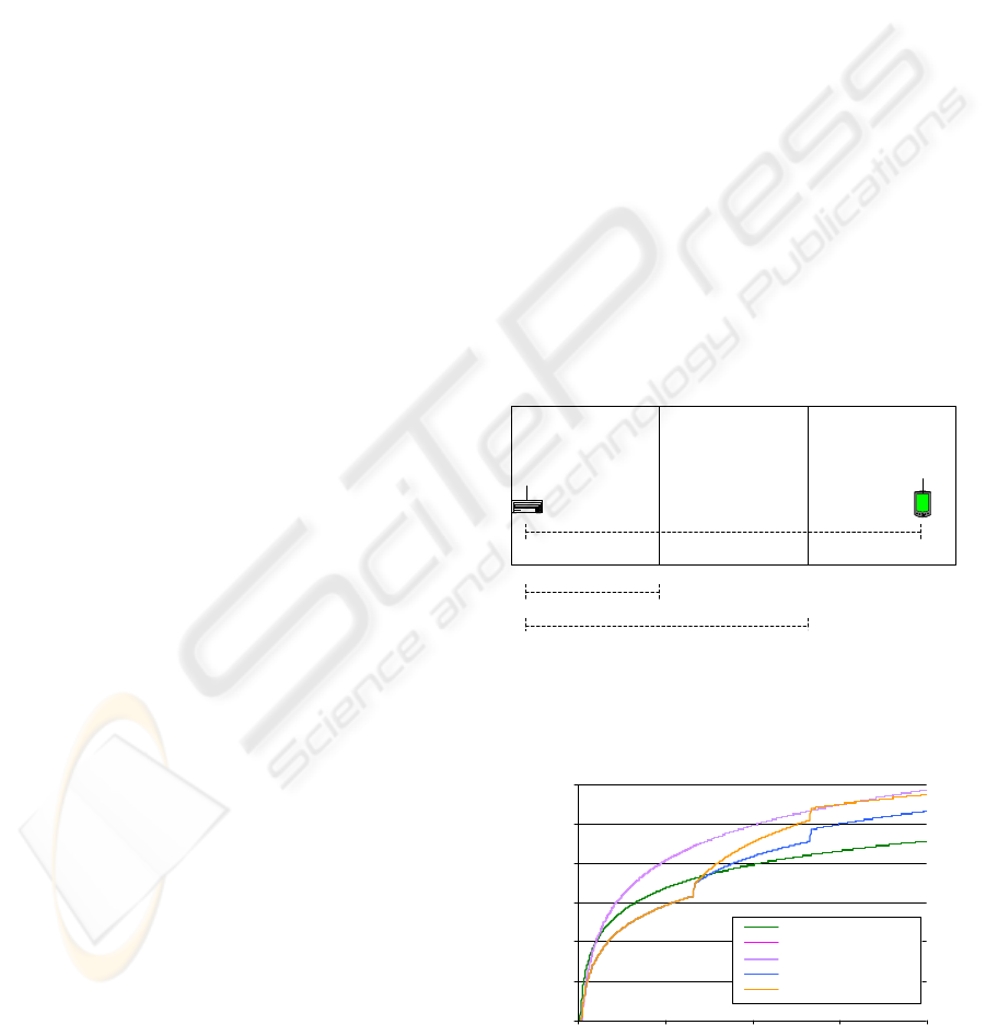
3 PROPOSED MODEL
In this Section a new model is proposed based on the
peculiarities of each of the models presented in
Section 2. All of them, except Keenan’s model,
introduce variable relations between distance and n,
depending on the environment. However the n value
presented by most of the models is general to a
building, not accounting for possible different rooms
crossed with different propagation conditions for
each (Figure 1). Considering these characteristics
and also the obstacles attenuation, it is possible to
maximize the best features of all models in one
single model. In (7) different rooms are taken into
consideration (propagation conditions), identifying it
with particular n for each and introducing the walls
and floors attenuation.
[] [ ]
(
)
[]
(
)
()
[]
()()
∑
=
+
+××−+
+
××
+
−
×
=
W
N
i
iiii
p
adnn
dnfL
1
m1
mMHzdB
log10
log1028log20
(7)
Where:
L – Proposed propagation model.
N
W
– Number of crossed walls.
n
p
– power decay index on point “p”, where the
attenuation is measured.
d
p
– distance between the transmitter and point “p”.
d
i
– distance between the transmitter and obstacle i.
n
i
– power decay index of room before obstacle i.
a
i
– obstacle i attenuation.
Transmitter
Receiver
Room 1 Room 2 Room 3
n
1
n
2
n
p
=n
3
d
p
d
1
d
2
Point p
Figure 1: Example for 3 rooms with different n values, and
2 obstacles (walls).
Figure 1 specifies the parameters of (7) and Figure 2
compares all presented models for the scenario
presented in Figure 1.
20
30
40
50
60
70
80
0 5 10 15 20
Distance [m ]
Attenuation [dB]
Free Space
One Slope Model
ITU
Keenan = COST231
Proposed Model
Figure 2: Propagation models comparison.
INDOOR PROPAGATION MODELS AND RADIO PLANNING FOR WLANS
89
4 MEASUREMENTS
Radio measurements were performed to characterize
n for different environments and also to obtain some
obstacles attenuation at 2.4GHz. Besides,
measurements are required to evaluate the models
performance (
Mikas, 2003). An AP was used as a
transmitter and a laptop computer with WLAN PCI
card antenna as a receiver, associated with
NetStumbler® tool.
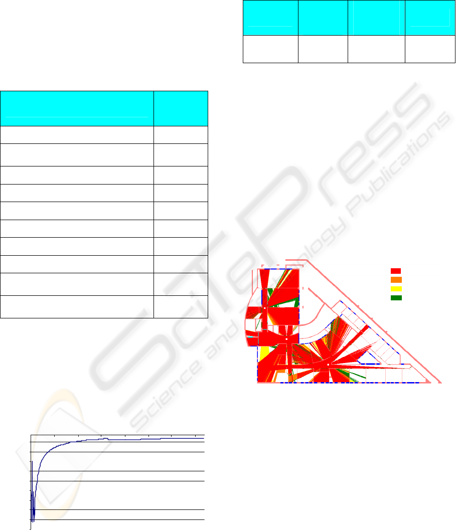
Table 1: Obstacles attenuation measurement
Obstacle
Atten.
[dB]
Wood door on a brick frame
6.64
Double wood door on a brick
frame
0.93
Fiber door
2.67
Simple glass window
4.48
Double glass window
6.40
Brick wall (14 cm)
11.80
Metal closet (1.5 m height)
14.43
Metal closet (2 m height)
23.64
Electromagnetic radiation
“shielded” wall
20.47
Concrete floor with false metal
ceiling
77.95
.
Phenomena listed in Section 2 cause fluctuations
on the signal’s power level, making it vary through
time around an average value. Therefore, it is
considered that each measure is concluded when the
number of power level samples is enough to
converge to its average as shown in Figure 3. This is
the loss value calculated by the models of Sections 2
and 3.
-52,5
-50,5
-48,5
-46,5
-44,5
-42,5
-40,5
-38,5
-36,5
-34,5
0 50 100 150 200 250 300 350
Number of Samples
Power Level [dBm]
Figure 3: Retrieving power level technique.
A set of “obstacles” were defined, being measured
their correspondent attenuation at 2.4GHz (Table 1).
Table 2: The n values for different scenarios
Alleyways
Class
rooms
Office
rooms
Labs
1.5 to 1.9 2.2 to 2.7 1.5 to 3.3 1.3 to 2.4
Table 2 presents n measurements, up to 4
different types of scenarios: alleyways, classrooms,
office rooms and electronics/computers equipment
laboratories (Labs).
5 PLANNING TOOL
The indoor planning tool, InPlanner, developed for
this study allows the following features: 2D display
of bit rate with different coverage areas (mapped by
colors), informing the exact percentage of occupied
area for each rate. Red for 11Mbit/s, orange for
5.5Mbit/s, yellow for 2Mbit/s and green for 1Mbit/s
(Figure 4).
11Mbit/s
5.5Mbit/s
2Mbit/s
1Mbit/s
Figure 4: Bit rate mapping.
The bit rate areas depend on power level and
Signal to Interference Ratio (SIR) on each point of
the plant (Figure 3). It also allows the estimation of
best server areas and C/I mapping. Besides coverage
estimation, this tool also estimates traffic load. It’s
possible to introduce office and student users
throughout the plant, distributed randomly or in
selected positions. It simulates: WWW, FTP, E-
Mail, Chat and video streaming, according to
CSMA/CA protocol.
To simulate E-Mail, FTP and video streaming,
an On/Off traffic source model is used. Each of
these packet services are considered continuous in
the same session. Once one of this services session’s
gets possession of the medium, it locks it until the
ICETE 2004 - WIRELESS COMMUNICATION SYSTEMS AND NETWORKS
90
session ends. WWW and Chat have a second level
of simulation. Being each session divided into
periods of data transfer and reading time (to
visualize the WWW pages and Chat messages
throughout the session). The service arrival process
is exponential distributed. Each service duration was
based on a campus local inquiry for students and
various office companies for office users. The
number of sub-sessions for WWW and Chat are
given by geometrical distribution and data volumes
by Pareto distribution (ETSI, 1998).
It outputs average delay for each AP on the
different floors. It uses the obstacles attenuations
(Table 2), the n values for different environments
(Table 1) and it allows to a user to choose the
propagation models, described in Section 2.
The propagation model can be chosen and all of
the parameters changed. Link Budget parameters
like the emitted power and antenna gains are
programmable, just like the receiver’s sensibility and
C/I limits. Also, all the average values for traffic
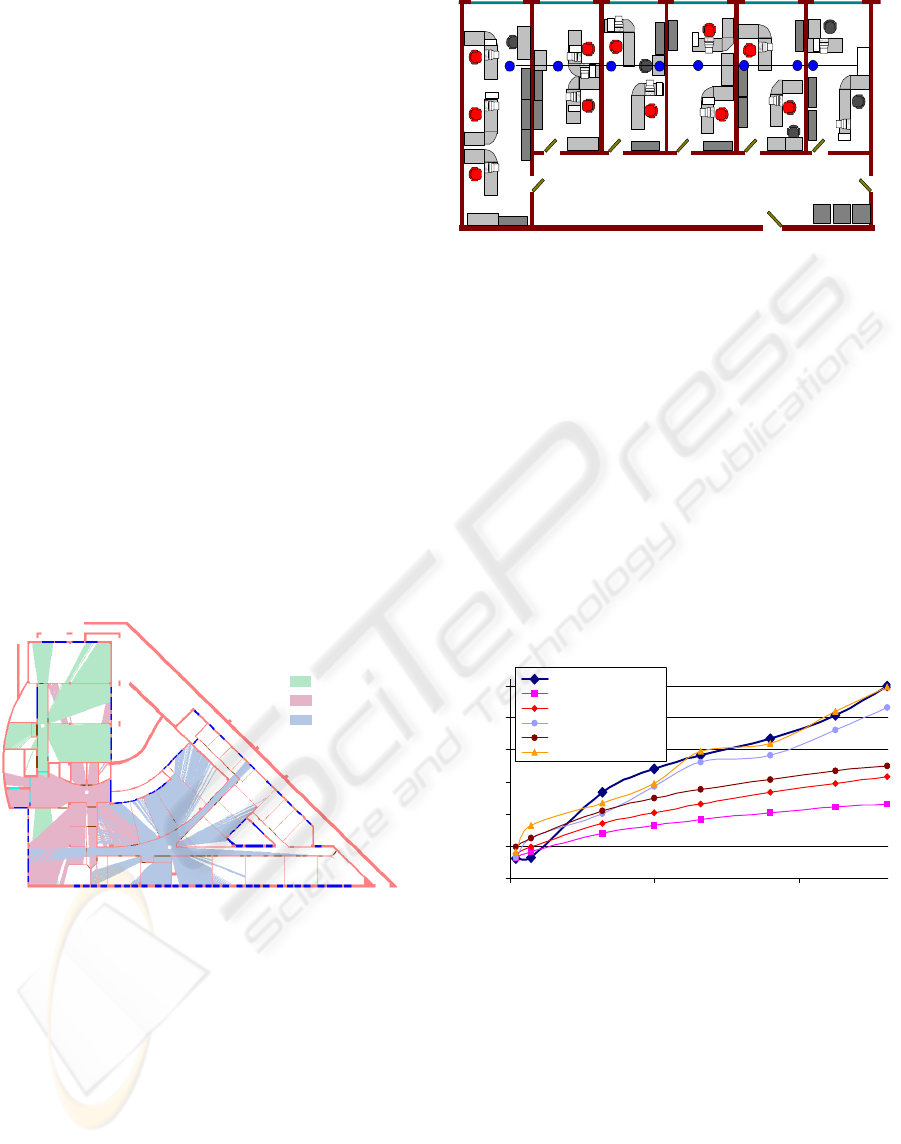
simulation are changeable. Figure 4 shows a view of
bit rate mapping with three APs. Figure 5
exemplifies how best server mapping is shown on
plant. Each color identifies the area covered by an
AP.
AP 1
AP 2
AP 3
Figure 5: Best server example.
6 ANALYSIS OF RESULTS
Using the results from measurements described in
Section 4, all the described models in Sections 2 and
3 are now put to test. Two typical examples are
considered to illustrate two measured scenarios. The
first one is an office area, with a link analysis
throughout 6 office rooms. Power levels are
measured in 8 points. The floor plant is shown in
Figure 6, where the measured points are represented
by blue dots.
A
P
Figure 6: Office Area (example 1).
The attenuation for each point is surpassed
using the Friis law. The proposed model considers
different n for each room and the walls attenuation,
which is shown in Table 1. Figure 7 contains the
attenuation curve for all models and also the
measured values for all points. The n value used in
all rooms for the proposed model is 2.5. One Slope
Model has n=3 and N for ITU is 30, being there the
recommended values for office environment, just
like α=0.57 for LAM model and n=2 (Mikas, 2003)
for COST 231.
As shown in Figure 8, the proposed model has
the better behavior on points 3, 4, 5, 6, 7 and 8. Point
1 is best modeled by Free Space, Keenan’s Model
and COST 231 model. Free Space Model has the
best approximation also for Point 2.
40
50
60
70
80
90
100
2712
Distance
[
m
]
Attenuation [dB]
Measured Values
Free Space
LAM
Keenan=COST
ITU=One Slope
Pro
p
osed Model
Figure 7: Comparision of all models (example 1).
Figure 8 represents the evolution of the
Absolute Error with distance for example 1. It can
be seen the significant improvement as the distance
and the number of obstacles increases. There is some
similarity with COST 231 and Keenan’s model, but
the differences are expected to be greater if the type
of environment would be more than one, like in this
example.
INDOOR PROPAGATION MODELS AND RADIO PLANNING FOR WLANS
91
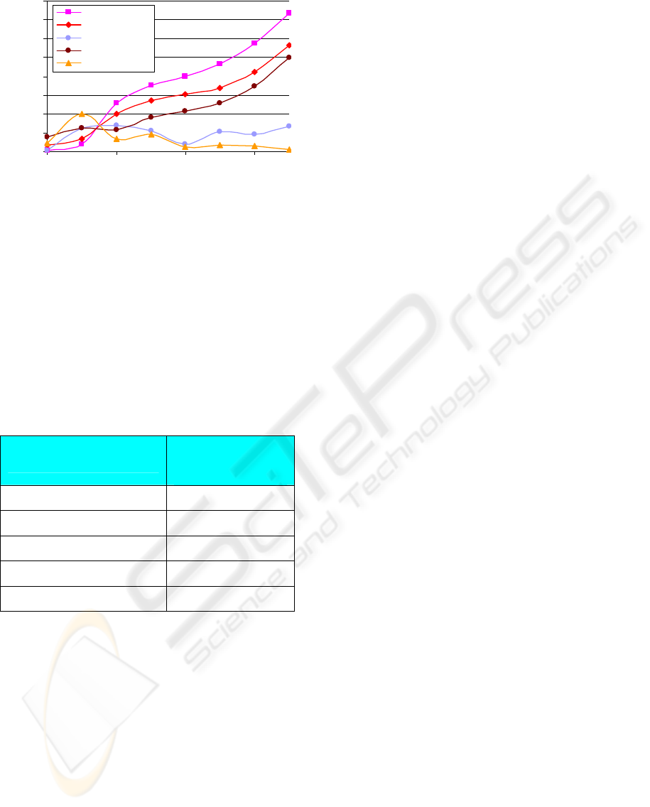
0
5
10
15
20
25
30
35
40
1357
Point Num be r
Absolute Error [dB]
Free Space
LAM
Keenan=COST
ITU=One Slope
Proposed Model
Figure 8: Absolute Error (example 1).
The second example represents a link with only
one point measured. The transmitter and the receiver
are separated by a fiber door (2.67dB attenuation)
between them. The transmitter is placed on an
electronics laboratory and the receiver on a class
room. The distance between the transmitter and the
door is 6.4m. The distance between the receiver and
the door is 2.28m.
Table 3 has the Absolute Error for all models.
The n value for One Slope and COST 231 and the N
value for ITU, as well as the α for LAM are defined
for office environment.
Table 3: Absolute Error for example 2
Propagation Model
Absolute Error
[dB]
One Slope and ITU
1.4
Proposed Model
1.6
LAM
2.9
Keenan and COST 231
5.2
Free Space
7.9
7 CONCLUSIONS
Despite the better results on shorter distances (not
relevant for coverage purposes), with one obstacle,
for One Slope and ITU model, the proposed model
has a good performance when compared with
measurements. Even in the long distance cases with
more than one obstacle between transmitter and
receiver (when different environments are crossed).
The developed planning tool InPlanner has the
capacity to implement this model and also to
perform traffic simulations, allowing coverage and
capacity planning.
This work stands as a contribution to the planning
methods required for the emerging technology of
WLANs. More tests must be carried out to evaluate
the proposed model with more different scenarios
(shopping malls, train stations and so on), with the
correspondent n index and other obstacles
attenuation determination.
The growing number of different applications
supported by WLANs, demands a continuous work
to improve the quality of radio planning. The
refining of the power decay index for the target
environments, as well as the determination of a large
number of obstacles attenuations should be
considered.
REFERENCES
Neskovic, A., Neskovic., N, and Paunovic, G., 2000.
Modern Approaches in Modeling of Mobile Radio
Systems Propagation Environment. In IEEE
Communications Surveys. The Electronic Magazine of
Original Peer-Reviewed Survey Articles.
Foerster, J., 2002. In IEEE P802.15 Working Group for
Wireless Personal Area Networks (WPANs), Channel
Modeling Sub-committee Report DRAFT. Intel
Research and Development.
Devasirvatham, D., Banerjee, C., Krain, M., and
Rappaport, D., 1990. In Multi-frequency radiowave
propagation measurements in the portable radio
environment. IEEE International Conference on
Communications.
Keenan, J., and Motley, A., 1990. In Radio coverage in
Buildings. Br.Telecom Technol.J.vol.8,no.1.
ITU-R P.1238-1, 1999. In Propagation data and
prediction methods for the planning of indoor
radiocommunication systems and radio local area
networks in the frequency range 900 MHz to 100 GHz.
Question ITU-R 211/3.
Tarokh, V., Ghassemzadeh, 2002. In S.S. The Ultra-
wideband Indoor Path Loss Model. IEEE
P802.15-02/277-SG3a and IEEE P802.15-02/278-
SG3a.
COST 231, 1999. In Digital Mobile Radio towards Future
Generation Systems.
Mikas, F., Zvánovec, S. and Pechac, P., 2003. In
Measurement and prediction of signal propagation for
WLAN systems. Department of Electromagnetic Field,
Czecalch Techni University.
ETSI, 1998. In Universal Mobile Telecommunications
System (UMTS); Selection procedures for the choice
of radio transmission technologies of the UMTS.
UMTS 30.03 version 3.2.0, Sophia Antipolis, France.
ICETE 2004 - WIRELESS COMMUNICATION SYSTEMS AND NETWORKS
92
