PACKET SCHEDULING FOR MAXIMIZING REVENUE IN A

NETWORK NODE

Jian Zhang, Timo H

ainen, Jyrki Joutsensalo

Dept. of Mathematical Information Technology

University of Jyv

askyl

a, FIN-40014 Jyv

askyl

a, Finland

Keywords:

Packet scheduling, QoS, pricing, revenue maximization.

Abstract:

In the future Internet, different applications such as Voice over IP (VoIP) and Video-on-Demand (VoD) arise

with different demands on Quality of Service (QoS). Different kinds of service classes (e.g. gold, silver,

bronze) should be supported in a network node. In the network node, packets are queued using a multi-

queue system, where each queue corresponds to one service class. The customers of different classes will pay

different prices to network providers based on multi-class pricing models. In this paper, we considered the

optimization problem of maximizing the revenue attained in a network node under linear pricing scenario. A

revenue-aware scheduling approach is introduced, which has the closed-form solution to the optimal weights

for revenue maximization derived from revenue target function by Lagrangian optimization approach. The

simulations demonstrate the revenue maximization ability of our approach.

1 INTRODUCTION

Integrated packet switched service networks must

carry a wide range of different trafﬁc types being

still able to provide performance guarantees to real-

time sessions such as Voice over IP (VoIP), Video-

on-Demand (VoD), or video-conferencing. Efﬁcient

and effective communication needs careful Quality of

Service (QoS) design in the future multi-service In-

ternet. In QoS design, different demands of different

types of trafﬁc classes (VoIP, VoD etc.) and different

prices paid by different classes (gold, silver, bronze

etc.) must be taken into account for giving plausible

and fair service.

Packet scheduling discipline is an important fac-

tor of a network node. The choice of the discipline

impacts the allocation of restricted network resources

among competing sessions of the communication net-

work. On the other hand, network operators can

handle resource reservations by using trafﬁc differ-

entiation and design different kind of pricing strate-

gies for customers with different service classes. The

open question still arises: how to put these two is-

sues together. Pricing research in the networks has

been quite intensive during the last few years (e.g.,

(Mackie-Mason et al, 1994), (Kelly, 1994), (Kelly,

1997), (Kelly et al, 1998), (Courcoubetis et al, 2000),

(Paschalidis et al, 2000), (La et al, 2002), (Pascha-

lidis et al, 2002)) and also novel fair scheduling algo-

rithms have been proposed (e.g., (Parekh et al, 1993),

(Golestani, 1994), (Stiliadis et al, 1995), (Stiliadis et

al, 1996)), but combination of them have not been an-

alyzed widely.

Our research differs from the above studies by link-

ing pricing and queuing issues together and allocat-

ing network resources among competing sessions in

the context of revenue maximization. In a network

node, packets are queued using a multi-queue sys-

tem, where each queue corresponds to one service

class. The customers of different classes will pay

different prices to network providers based on multi-

class pricing models. In this paper, we considered

the optimization problem of maximizing the revenue

attained in a network node under linear pricing sce-

nario. A revenue-aware scheduling approach is intro-

duced, which has the closed-form solution to the op-

timal weights for revenue maximization derived from

revenue target function by Lagrangian optimization

approach. The simulations demonstrate the revenue

maximization ability of our approach.

The rest of the paper is organized as follows. In

Section 2, three pricing scenarios (linear, ﬂat and

piecewise linear) are presented and the linear one

is generally deﬁned. Revenue-aware scheduling ap-

134

Zhang J., Hämäläinen T. and Joutsensalo J. (2004).

PACKET SCHEDULING FOR MAXIMIZING REVENUE IN A NETWORK NODE.

In Proceedings of the First International Conference on E-Business and Telecommunication Networks, pages 134-139

DOI: 10.5220/0001392601340139

 SciTePress

. . .

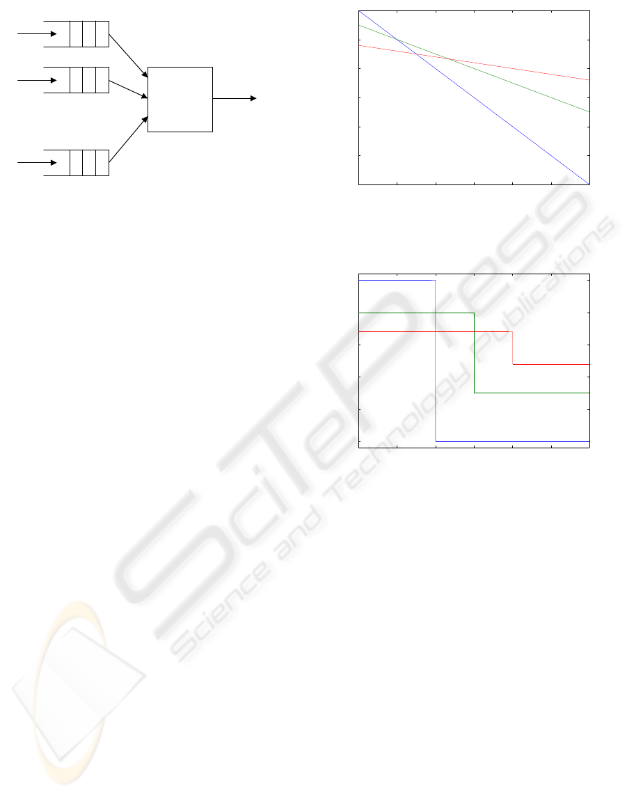
CLASS 1

CLASS 2

CLASS m

w1

w2

wm

OUTPUT

lambda 1

lambda 2

lambda m

PACKET

SCHEDULER

Figure 1: Trafﬁc classiﬁcation at the packet scheduler

proach is derived in Section 3, where the closed-

form solution to the optimal weights is presented in

the context of revenue maximization and the analytic

maximum revenue is also derived. Section 4 contains

simulation part demonstrating the revenue maximiza-

tion ability of our approach. Finally, in Session 5, we

present concluding remarks.

2 PRICING SCENARIO

Here three simple pricing scenarios are presented and

we believe that they are also the most used ones. First

some parameters and notions are deﬁned. Let d

be the minimal processing time of the scheduler for

transmitting 1-bit data from one queue to the output in

Fig. 1, i.e., d

= 1/C if the processing capacity of the

scheduler is C bits/s. The number of service classes

is denoted by m. Literature usually refers to the gold,

silver and bronze classes; in this case, m = 3. The

mean delay for class i during one measurement pe-

riod is referred to as

. For each service class, a pric-

ing function r

(

) will be deﬁned to rule the relation-

ship between the QoS provided by network providers

(mean delay in this case) and the payment of their cus-

tomers (revenue/penalty in this paper). Obviously, it

is non-increasing with respect to its mean delay

Examples of pricing functions are given in Figs. 2, 3,

and 4, which show the most used pricing strategies:

linear, ﬂat and piecewise linear models, respectively.

In this paper, our study concentrates on the revenue-

maximizing issue under linear pricing functions and

the analysis under ﬂat pricing strategy is postponed to

its sequel. The solution to the piecewise linear pricing

model is a straightforward extension to the above two

ones. Speciﬁcally, Linear pricing model for class i is

characterized by the following deﬁnition.

Deﬁnition 1: The function

(

) = b

− k

, i = 1, 2, ..., m, b

> 0, k

> 0

(1)

0 10 20 30 40 50 60

−400

−300

−200

−100

100

200

mean delay

revenue

Linear pricing functions

Figure 2: Three linear pricing functions. Horizontal axis:

mean delay; vertical axis: price.

0 10 20 30 40 50 60

−150

−100

−50

100

mean delay

revenue

Flat pricing functions

Figure 3: Three ﬂat pricing functions. Horizontal axis:

mean delay; vertical axis: price.

is called linear pricing function, where b

and k

are

positive constants and normally b

≥ b

and k

≥

hold to ensure differentiated pricing if class i has

higher priority than class j (in this paper, we assume

that class 1 is the highest priority and class m is the

lowest one).

Fig. 2 depicts three linear pricing functions for

gold, silver and bronze classes and it is commented

more detailed below. For gold class, the pricing func-

tion r

(

) = 200 − 10

means that when its mean

delay

is small, the price paid by gold class cus-

tomers is high - in this case, maximally 200 units

of money. It is natural that for the highest priority

class, constant shift b

is selected to be the highest.

On the other hand, penalty paid to the highest pri-

ority class customers is also highest if the scheduler

fails to meet its minimum requirement of mean delay

(20 time units in this case) and the growing rate of

penalty along with mean delay depends on the slope

(highest in this case). For example, if

= 30,

then r

(

) = r

(30) = 200 − 10 ∗ 30 = −100,

i.e., the penalty is 100 units of money. Same obser-

PACKET SCHEDULING FOR MAXIMIZING REVENUE IN A NETWORK NODE

135

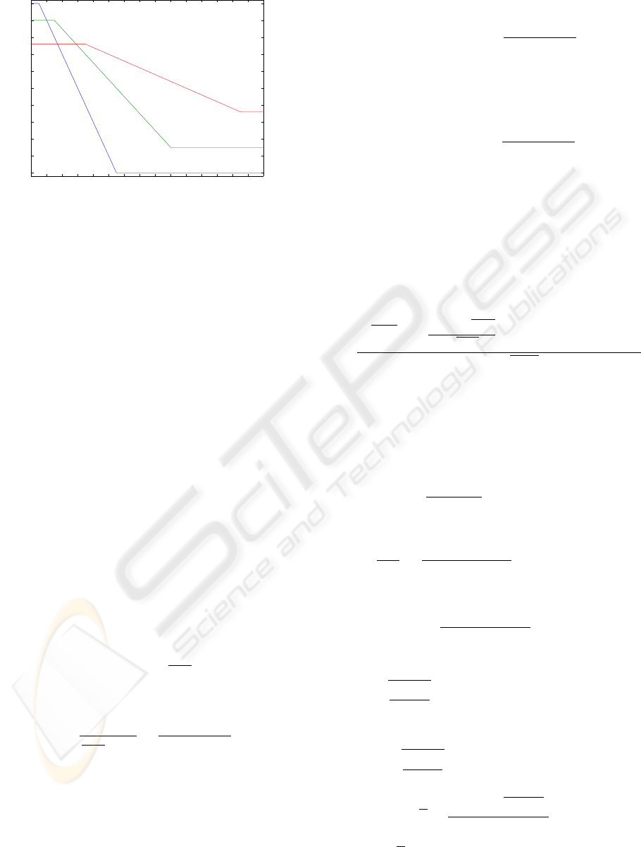
0 10 20 30 40 50 60 70 80 90 100 110 120 130 140 150

−300

−250

−200

−150

−100

−50

100

150

200

mean delay

revenue

Piecewise linear pricing functions

Figure 4: Three piecewise linear pricing functions. Hori-

zontal axis: mean delay; vertical axis: price.

vations hold for silver and bronze classes. For bronze

class, r

(

) = 80 −2

means that the price paid by

that class customers is maximally 80 units of money.

In this case, constant shift b

is lowest. On the other

hand, the growing rate of penalty for bronze class will

also be lowest since its slope k

= 2 is the lowest.

3 REVENUE MAXIMIZATION

APPROACH

Let us consider a packet scheduler fed by m Poisson

streams with arrival rates λ

, λ

, ..., λ

as shown in

Fig. 1. We assume that in this paper the distribution

of packet length in all classes is exponential and use

to denote the mean packet size in bits in class i.

Let the weight allotted to class i be w

, i = 1, 2, ..., m.

Without loss of generality, only non-empty queues are

considered, and thus w

6= 0. If some weight w

= 1,

then m = 1. Therefore, the natural constraint for the

weights is

i=1

= 1, w

∈ (0, 1]. If the weight

assigned to class i is w

, class i in the scheduler can

be guaranteed to have a share of processing capac-

ity w

(bits/s) and mean service time of packets

in class i can be estimated by

; hence, the ana-

lytic form of mean delay

for class i packet can be

denoted as

− λ

(2)

based on queueing theory. The natural constraint for

Eq. (2) is w

> λ

due to the fact that delay can

not be negative.

We use the analytic form

in Eq. (2) to estimate

the real mean delay of class i packet

during one

measurement period and deﬁne F to be the revenue

gained in a network node during that period as follows

when the linear pricing function in Eq. (1) is used:

F =

i=1

(

) =

i=1

−

− λ

) (3)

As a result of the above deﬁnition, the issue of rev-

enue maximization in a packet scheduler can be for-

mulated as follows:

max F =

i=1

−

− λ

) (4)

s.t.

i=1

= 1, 0 < w

≤ 1 (5)

> λ

(6)

Theorem 1 For linear pricing functions, the globally

maximum revenue F is achieved by using the follow-

ing optimal weight

(1 +

j=1

√

−

j=1

)

j=1

i = 1, 2, ..., m (7)

and it is unique when w

∈ (0, 1].

Proof: Based on Equations (4) and (5), we can con-

struct the following Lagrangian equation.

P = P (w

, w

, ..., w

)

i=1

−

−λ

) + σ(1 −

i=1

) (8)

Set partial derivatives of P in Eq. (8) to zero:

∂P

∂w

− λ

)

− σ = 0. (9)

It follows that

σ =

− λ

)

(10)

leading to the solution

+ λ

, i = 1, 2, ..., m. (11)

Substituting Eq. (11) to Eq. (5), we get

i=1

= 1

√

σ =

i=1

1 −

i=1

(12)

And when

√

σ in Eq. (12) is substituted to Eq. (11),

the closed-form solution in Eq. (7) is obtained.

ICETE 2004 - SECURITY AND RELIABILITY IN INFORMATION SYSTEMS AND NETWORKS

136

Because of the constraint in Eq. (6) w

> λ

obviously,

j=1

= 1 >

j=1

(13)

Hence, the closed-form solution in Eq. (7) w

> 0.

Moreover, based on (13), the following inequality

holds

−

j6=i

j=1

j6=i

j=1

≤ 1

leading to in Eq. (7) the numerator less than the de-

nominator. Hence, we can conclude that 0 < w

≤ 1.

To prove that the closed-form solution in Eq. (7)

is the only and optimal one in the interval (0, 1], we

consider second order derivative of P.

∂

∂w

= −

− λ

)

< 0 (14)

due to the constraint w

> λ

in (6). Therefore,

the revenue F gained by a network provider is strictly

concave in the interval 0 < w

≤ 1, having one

and only one maximum. This completes the proof.

Q.E.D.

Analytical form of the maximum revenue gained

during a measurement period can be expressed by the

optimal weights given in Eq. (7).

Theorem 2 When the optimal weights are used ac-

cording to Theorem 1, the analytic value of maximum

revenue obtained in a network node during the mea-

surement period is

max

i=1

−

(

i=1

)

1 −

i=1

(15)

Proof: When the optimal weights in Eq. (7) are sub-

stituted to Eq. (3), the maximum revenue obtained is

max

i=1

−

i=1

(1 −

i=1

)

i=1

−

i=1

1 −

i=1

)

i=1

−

(

i=1

)

1 −

i=1

Q.E.D.

4 SIMULATIONS

In this section we present some simulation results to

illustrate the effectiveness of our approach for max-

imizing revenues under linear pricing functions. A

number of simulations have been conducted under

different parameter settings. In each case, we numer-

ically determine the optimal solutions using Theorem

1 and 2, and then we investigate through simulation

the beneﬁts of our approach by comparing the rev-

enues obtained under our optimal weights with those

obtained under a natural scheme of proportional as-

signment. A representative set of these simulations

are presented herein. Throughout this section, we

shall focus on a packet scheduler with the number

of service classes m = 3 (namely, gold, silver and

bronze classes) and minimum processing time d

−6

s. The base arrival rates and the mean packet

sizes for three classes are provided in Table 1. A mul-

tiplicative load factor ρ > 0 is used to scale these

base arrival rates to consider different trafﬁc intensi-

ties; i.e., λ

ρ is used in the simulations for class-j ar-

rival rate. As previously noted, we use a scheme that

proportionally allocates the weight among all service

classes for comparison with our revenue-maximizing

approach. Speciﬁcally, the proportional scheme as-

signs the weight for class i as follows:

j=1

(λ

)

, i = 1, 2, ..., m. (16)

Note that this proportional assignment scheme is a

natural way to allocate the scheduler processing ca-

pacity.

Table 1: The base parameters for packet trafﬁc

i = 1 i = 2 i = 3

(gold class) (silver class) (bronze class)

10 15 20

(packets/s)

(bits)

3360 3360 3360

4.1 The ﬁrst set of simulations

In the ﬁrst set of simulations, the parameters related

to three linear pricing functions used are summarized

as follows: b

= 200, k

= 10000, for gold class,

= 150, k

= 5000, for silver class, and b

= 80,

= 2000, for bronze class (note that the time unit is

second here).

First we investigate the evolution of the revenue

along with the time under our optimal weights and

the proportional weights. In this case, the base arrival

rates in Table 1 are used and one set of given weights

= 0.60, w

= 0.25, w

= 0.15) is also used

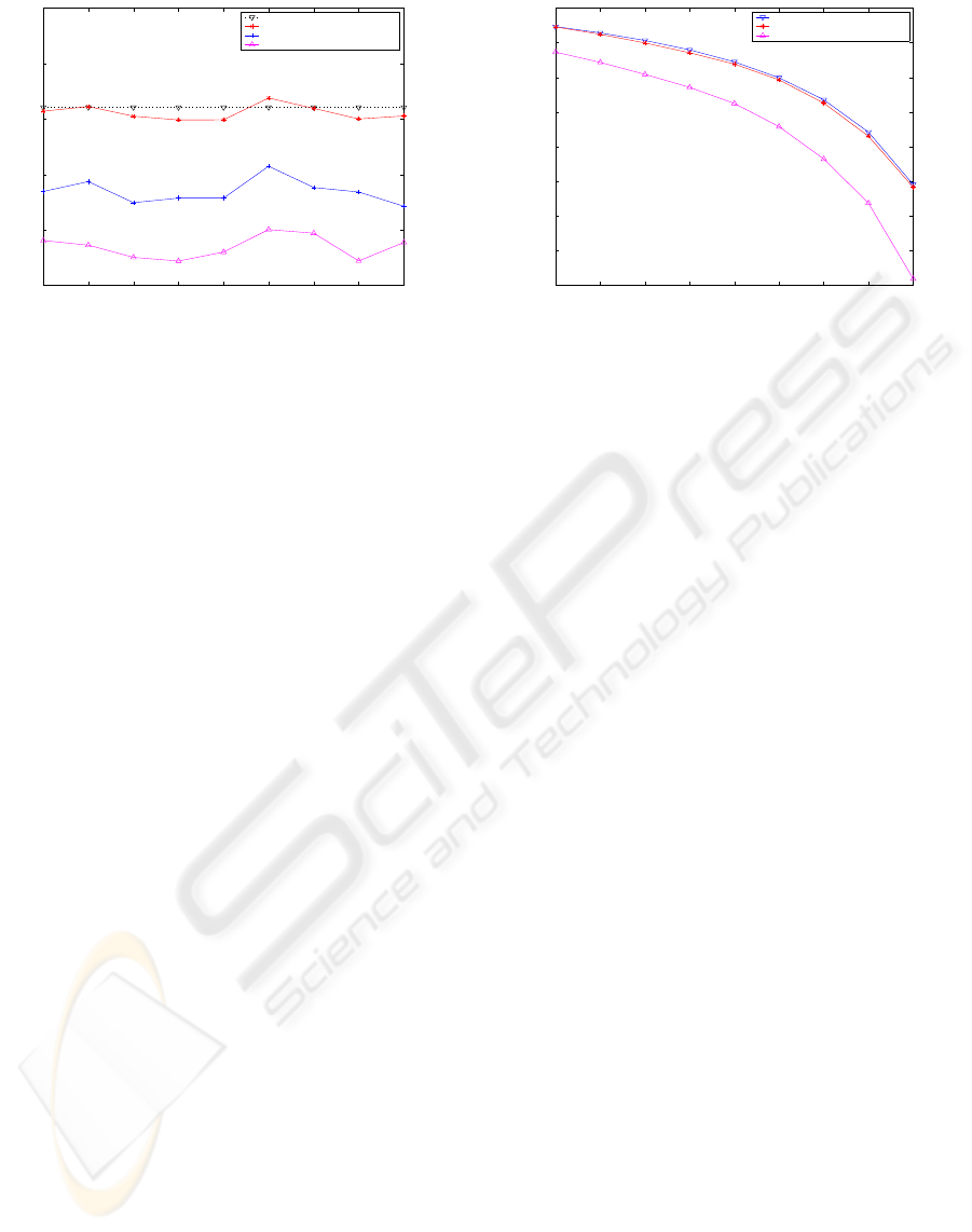
for comparison with our approach. Fig. 5 presents

the simulation results, where the x-axis represents the

time (the measurement period is 100 seconds here)

and the y-axis represents the revenue obtained during

PACKET SCHEDULING FOR MAXIMIZING REVENUE IN A NETWORK NODE

137

100 200 300 400 500 600 700 800 900

150

180

210

240

270

300

time (s)

revenue

Analytic

Simulated under optimal weights

Simulated under given weights

Simulated under proportional weights

Figure 5: Revenue comparison as function of time, for the

case, load factor ρ = 1 and b

= 200, k

=10000, b

= 150,

= 5000, b

= 80, k

= 2000.

that measurement period. Unless stated otherwise, we

shall hereafter refer to the latter as revenue. It is ob-

served that the largest revenue is achieved under our

optimal weights compared with those achieved un-

der the proportional and given weights and it is quite

close to the analytic value of maximum revenue by

Eq. (15). Since the parameters used in Eq. (15) are

constant in this case, the analytic value remains con-

stant; whereas, for the mean delay of packets by simu-

lations is variable, the simulated revenue varies along

with the time. Fig. 5 shows that the revenue obtained

under our optimal weights is very close to the ana-

lytic value, which demonstrates the effectiveness of

our approach for revenue maximization.

Next we examine the performance of our revenue-

maximizing approach for the case that the same pric-

ing functions are used and different trafﬁc intensi-

ties are fed into the packet scheduler. Fig. 6 shows

the simulation results, where the x-axis represents the

load factor and the y-axis represents the revenue.

First focusing on our revenue-maximizing ap-

proach, we can see that the revenues obtained under

our optimal weights are extremely close to those of

analytic forms for light and medium loads, and both

decrease along with the load factor. This is as ex-

pected because the increase of the trafﬁc load fed into

the scheduler incurs the increase of the mean delay

and thus the decrease of the obtained revenue. At

heavier loads both curves start to level off sharper

as the penalties start to grow faster. Compared with

our approach, the proportional assignment scheme

achieves less revenues at all trafﬁc loads. And it de-

creases even sharper for heavier load as the penal-

ties incurred under the proportional weights are much

larger than the ones under our optimal weights for the

same load and grow faster.

1 1.5 2 2.5 3 3.5 4 4.5 5

−500

−400

−300

−200

−100

100

200

300

Load factor

revenue

Analytic

Simulated under optimal weights

Simulated under proportional weights

Figure 6: Revenue comparison as function of load factor ρ,

for the case, b

= 200, k

=10000, b

= 150, k

= 5000,

= 80, k

= 2000.

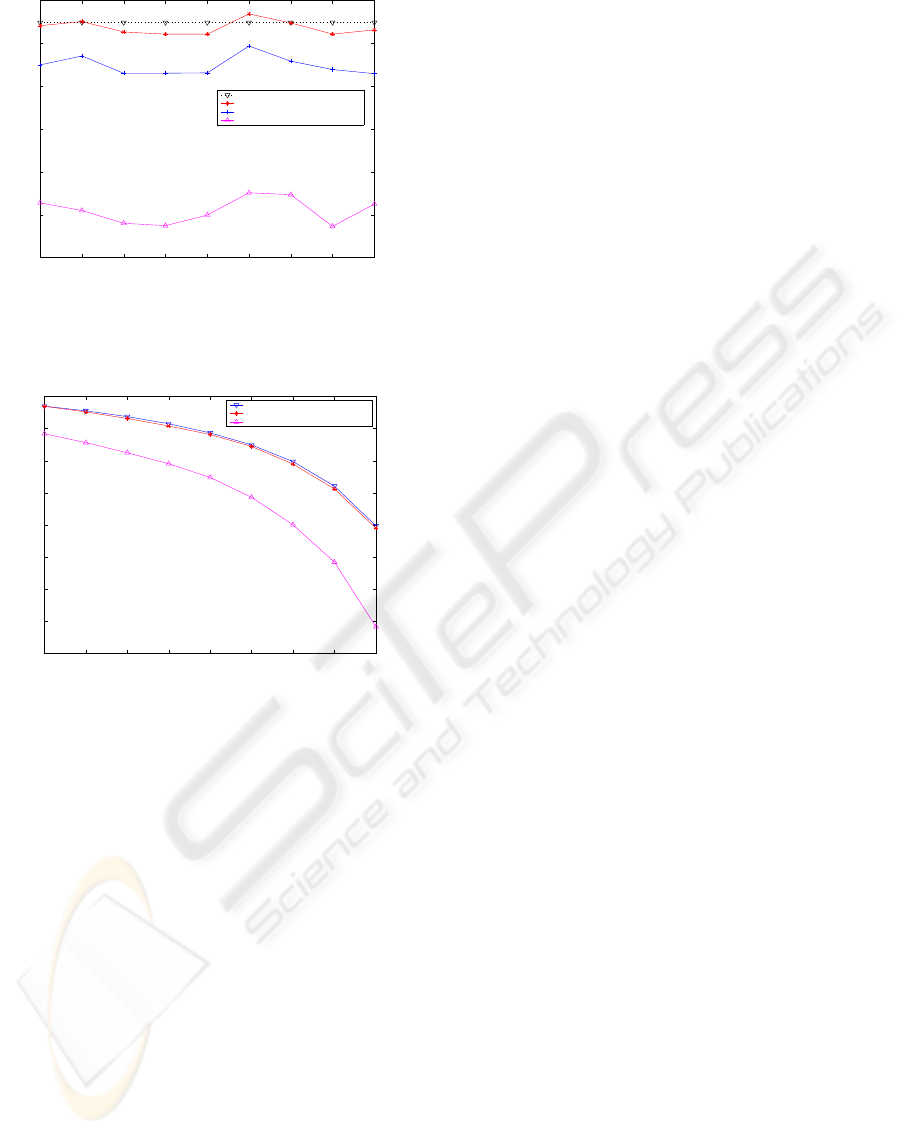
4.2 The second set of simulations

In the second set of simulations, the same simulations

are made for three different linear pricing functions:

= 200, k

= 5000, for gold class, b

= 120, k

2000, for silver class, and b

= 40, k

= 500, for

bronze class, to evaluate the performance robustness

of our approach for revenue maximization. Figs. 7

and 8 present the simulation results.

It is observed in Fig. 7 that the revenue obtained

under our optimal weights is the largest and it is also

close to the analytic value by Eq. (15). Since the slope

of class i in this case is less than the one in the ﬁrst

set of simulations, the revenue obtained from class i

will decrease more slowly along with the increase of

mean delay in this case, leading to the revenue curves

in Fig. 8 level off smoother for the same load com-

pared with the ones in Fig. 6. Similarly, the largest

revenue is obtained under our optimal weights for all

trafﬁc loads and it is very close to the curve of analytic

maximum revenue. Therefore, it is demonstrated that

our revenue-maximizing approach is effective for any

linear pricing functions.

5 CONCLUSIONS

In this paper, we explored the problem of max-

imizing revenues under multi-class Service-Level-

Agreements. In particular, we considered the opti-

mization problem of maximizing the revenue attained

in a network node under linear pricing scenario. A

revenue-aware scheduling approach was introduced,

which has the closed-form solution to the optimal

weights for revenue maximization derived from rev-

enue target function by Lagrangian optimization ap-

proach. The simulations demonstrated the revenue

maximization ability of our approach.

ICETE 2004 - SECURITY AND RELIABILITY IN INFORMATION SYSTEMS AND NETWORKS

138

100 200 300 400 500 600 700 800 900

230

240

250

260

270

280

290

time (s)

revenue

Analytic

Simulated under optimal weights

Simulated under given weights

Simulated under proportional weights

Figure 7: Revenue comparison as function of time, for the

case, load factor ρ = 1 and b

= 200, k

=5000, b

= 120,

= 2000, b

= 40, k

= 500.

1 1.5 2 2.5 3 3.5 4 4.5 5

−100

−50

100

150

200

250

300

Load factor

revenue

Analytic

Simulated under optimal weights

Simulated under proportional weights

Figure 8: Revenue comparison as function of load factor ρ,

for the case, b

= 200, k

=5000, b

= 120, k

= 2000,

= 40, k

= 500.

In the future work, the issue of revenue maximiza-

tion for ﬂat pricing scenario is investigated. More-

over, revenue criterion may be used as an admission

control mechanism. In admission control, the packet

is accepted/rejected by hypothesis test, where revenue

increase/decrease is estimated, when a packet comes.

REFERENCES

Courcoubetis C., Kelly F.P., and Weber R. (2000).

Measurement-based usage charges in communication

networks.

Oper. Res.. Vol.48, No.4, pp. 535-548, 2000.

Golestani S.J. (1994).

A Self-Clocked Fair Queuing Scheme for Broadband

Applications

In Proc. of INFOCOM’94, pp. 636-646, April 1994.

Kelly F.P. (1994).

On tariffs, policing and admission control for multi-

service networks.

Oper. Res. Lett.. Vol.15, pp. 1-9, 1994.

Kelly F.P. (1997).

Charging and rate control for elastic trafﬁc.

European Transaction on Telecommunication, Vol.8,

pp. 33-37, 1997.

Kelly F.P., Maulloo A.K., and Tan D.K.H. (1998).

Rate control for communication networks: Shadow

prices, proportional fairness and stability.

Oper. Res. Soc., Vol.49, pp. 237-252, 1998.

La R.J. and Anantharam V. (2002).

Utility-based Rate Control in the Internet for Elastic

Trafﬁc.

IEEE/ACM Transactions on Networking, Vol.10, Is-

sue: 2, pp. 272-286, April 2002.

MacKie-Mason J.K. and Varian H.R. (1994).

Pricing the Internet, in Public Access to the Internet.

B. Kahin and J. Keller, Eds. Englewood Cliffs, NJ:

Prentice-Hall, 1994.

Parekh A.K. and Gallager R.G. (1993).

A Generalized Processor Sharing Approach to Flow

Control in Integrated Services Networks: The

Single-Node Cases.

IEEE/ACM Transactions On Networking, Vol.1, No.3,

pp. 344-357, June 1993.

Paschalidis I.Ch. and Tsitsiklis J.N. (2000).

Congestion-dependent pricing of network services.

IEEE/ACM Transactions on Networking, Vol.8, pp.

171-184, April 2000.

Paschalidis I.Ch. and Liu Y. (2002).

Pricing in multiservice loss networks: static pricing,

asymptotic optimality and demand

subsitution effects.

IEEE/ACM Transactions on Networking, Vol.10, Is-

sue: 3, pp. 425-438, June 2002.

Stiliadis D. and Varma A. (1995).

Efﬁcient Fair Queuing Algorithm for ATM and Packet

Networks.

Tech. Rep. UCSCCRL-95-59, Dec. 1995.

Stiliadis D. and Varma A. (1996).

Design and Analysis of Frame-based Fair Queuing: A

New Trafﬁc Scheduling Algorithm for

Packet-Switched Networks.

In Proc. of SIGMETRICS’96, pp. 104-115, May 1996.

PACKET SCHEDULING FOR MAXIMIZING REVENUE IN A NETWORK NODE

139