
RELIABILITY ASSESSMENT OF E-COMMERCE APPLICATIONS
V. S. Alagar
Concordia University
Montreal, Quebec, Canada
O. Ormandjieva
Concordia University
Montreal, Quebec, Canada
Keywords:
E-Commerce, reliability prediction, software measurement, Markov model.
Abstract:
The paper discusses a formal approach for specifying time-dependent E-Commerce applications and proposes
a Markov model for reliability prediction. Measures for predicting reliability are calculated from the formal
architectural specification and system configuration descriptions. Our methods have been implemented and a
set of sample results obtained from it for a simple system is given.
1 INTRODUCTION
The reliability of a software system is defined in
(IEE, ) as the ability to perform the required function-
ality under stated conditions for specified period of
time. In this paper the software system under discus-
sion is an E-Commerce system. An E-Commerce can
be viewed as a large and complex distributed system
whose heterogeneous components interact in various
ways to achieve the result of an application. Often,
the performance of an application initiated at a site is
rated as good if the server at that site is robust and
maintains its links to other web objects throughout a
transaction session. Such a rating does give a sub-
jective qualitative assessment, but does not provide a
scientific quantitative measurement of the reliability
of the site or the system itself. This paper proposes a
rigorous methodology for predicting the reliability of
E-Commerce applications using Markov models con-
structed from a formal model of the E-Commerce ap-
plication.
Many techniques exist to test and statistically an-
alyze traditional software. However, these methods
can not be readily applied to E-Commerce systems.
In a recent paper Kallepalli and Tian (Kallepalli and
Tian, 2001) have surveyed the characteristics of Web
applications and usage and proposed a statistical test-
ing method for Web applications. Their approach
relies on usage and failure information collected in
the log files. They define Web failure as the inabil-
ity to correctly deliver information or documents re-
quired by the users. Based on this definition of failure,
they classify types of failures and provide a method
for testing source or content failures. We comple-
ment and enrich this work by offering a formal time-
constrained model of a simple E-Commerce model.
We propose an early reliability prediction based on
the analysis of the formal architecture model of the
E-Commerce applications using Markov models. A
Markov model dynamically adapts to time-dependent
system configurations that satisfy the architectural de-
sign (Ormandjieva, 2002). We view the E-Commerce
applications as large Markov systems, in which state
changes within each object of the system occur with
certain probabilities.
Following the work (Papazoglou, 2000), we use
agent paradigm to formally model E-Commerce sys-
tems. Agents are usually qualified by their goals,
knowledge, beliefs, and intentions. We follow the
property-oriented definition and classification from
(Alagar et al., 2002), and introduce primitive agent
types in modeling an E-Commerce system.
The organization of the rest of the paper is as fol-
lows. A formal model of the E-Commerce is given
in Section 2. Section 3 formally describes the
method of modeling the E-Commerce application as
a Markov system. Section 4 presents the reliability
prediction measures obtained from our implementa-
tion for a simple system. Section 5 concludes the
paper with a discussion on our ongoing research di-
rections.
30
S. Alagar V. and Ormandjieva O. (2004).
RELIABILITY ASSESSMENT OF E-COMMERCE APPLICATIONS.
In Proceedings of the First International Conference on E-Business and Telecommunication Networks, pages 30-37
DOI: 10.5220/0001399900300037
Copyright
c
SciTePress
2 E-COMMERCE MODEL
In this paper, an agent is a computational entity han-
dling sequences of messages (events) to implement
the expected behavior of an agent as understood in
agent technology (FIP, ; Papazoglou, 2000). Agents
can receive and emit events, generate events inter-
nally, and react to events received from its environ-
ment. Such handling is fully determined by the im-
plementation of the event. Peer-to-peer communica-
tion between agents is enabled by bidirectional con-
nections transmitting events according to a speci-
fied protocol. We refer to (Franklin and Graesser,
1996; Alagar et al., 2002) for agent classification,
agent types, agent behaviors, and their conformance
to FIPA agents. We use the notation from (Alagar
et al., 2002) for describing an E-Commerce system.
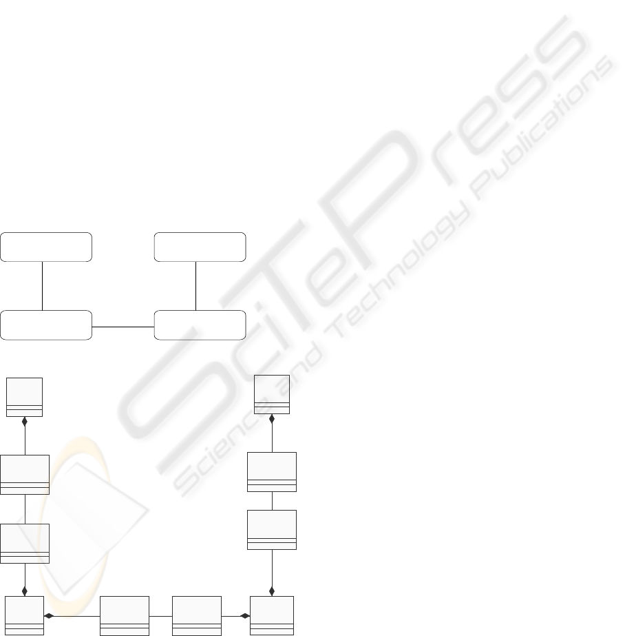
For illustration, we develop the formal model of an
E-Commerce system consisting of four agent types
User, EBroker, Merchant, and Bank. An instance
of an agent type is an agent. The high-level architec-
ture shown in Fig. 1(a) captures the allowed connec-
tions between agents in an application.
User
EBroker
Bank
Merchant
(a) Generic E-Commerce Architecture
User
(f rom U ser)
<<GRC>>
@A
(from User)
<<PortType>>
@U
(f rom EBroker)
<<PortType>>
EBroker
(f rom EBroker)
<<GRC>>
@C
(f rom EBroker)
<<PortType>>
@G
(f rom Merchant)
<<PortType>>
Merchant
(f rom Merchant)
<<GRC>>
@B
(f rom Merchant)
<<PortType>>
@M
(from Bank)
<<PortType>>
Bank
(f rom Bank)
<<GRC>>
(b) Agent Types and Port Types
Figure 1: High-Level Architecture Diagrams
2.1 Formal Models
From the architecture shown in Fig. 1(a) we deter-
mine the agent types and port types for each agent
type. A port-type of an agent type [] is an abstrac-
tion of connection point where events are emitted
and received from another agent type. The symbol
@ is used to introduce port types. An agent of the
agent type A[L], where L is the list of port types,
is created by instantiating each port type in L by
a finite number of ports and assigning the ports to
the agent. Any message defined for a port type can
be received or sent through any port of that type.
For instance, A
1
[p
1
, p
2
: @P ; q
1
, q
2
, q
3
: @Q], and
A
2
[r
1
: @P ; s
1
, s
2
: @Q] are two agents of the agent
type A[@P, @Q]. The agent A
1
has two ports p
1
and
p
2
of type @P , and three ports q
1
, q
2
, q
3
of type @Q.
Both p
1
and p
2
can receive or send messages of type
@P ; the ports q
1
, q
2
, and q
3
can receive and send
messages of type @Q. Sometimes the port param-
eters of agents are omitted in our discussion below.
Messages are allowed to have parameters.
An E-Commerce system, consistent with the archi-
tecture in Figure 1(a), consists of a finite set A of
agents A
1
, . . . A
n
, where each A
i
is an instance of one
of the agent types shown. From the description of the
problem we extract the messages (events) for commu-
nication and partition the set of the messages into co-
hesive subsets, creating port-types. For instance, the
EBroker agent type requires two port types: one for
communication with the User agent and the other for
communication with the Merchant agent. Figure 1(b)
shows a refinement of Figure 1(a) obtained by adding
the port type associations to agent types. The model
is further enriched by including abstract data types to
express abstract computations done by agents.
2.2 Behavior of the System
An agent can handle one external event at a time. We
assume that there is no connection delay, and an agent
emits an event only if the receiver of the event is pre-
pared to accept it. That is, emitting and absorbing an
event is considered as one atomic action. Thus, in a
specific transaction in the system, the activity of each
agent A on a set of connections C is observed as the
finite sequence of events which A handles on C in that
session. Notice that the connections C are at the ports
of A and the ports of those agents interacting with it in
that session. The trace of A on C is the set of all com-
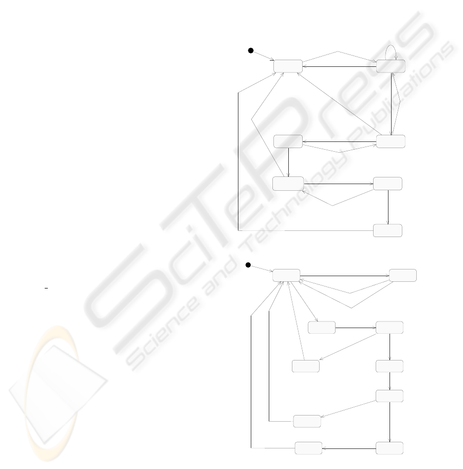
putation paths in the state machine description of A.
The set of all traces of A is referred to as the behav-
ior of A. Fig. 2 and Fig. 3 show the state machines
for the agents in our E-Commerce system. To illus-
trate the usefulness of time constraints we have spec-
ified time constraints for EBroker actions. In general
RELIABILITY ASSESSMENT OF E-COMMERCE APPLICATIONS
31
Merchant and Bank agents should also respect time-
liness, and appropriate time constraints can be intro-
duced in their specifications.
A successful transaction is conducted by the agents
in the following manner. The E-Commerce system
is initiated with the message BrowseAdd from a user
to the broker. Both User and EBroker agents syn-
chronize on this event: the agent User goes to active
state, the agent EBroker goes to the state getProd-
uct. The other agents do not change their states. The
agent EBroker sends the message GetProductInfo to
the Merchant agent within 2 units of time from the
instant of receiving the message BrowseAdd, and they
both simultaneously change their states to waitProd-
uct, and product respectively. The Merchant agent
responds to the agent EBroker with the message Pro-
ductInfo which cause them to simultaneously change
their states to idle, and browseSucceed. Within 2 units
of time of receiving the webpage from the merchant
the EBroker communicates to the User agent with
the message page, causing them to simulataneously
change their states to idle and readPage. This com-
pletes the first phase of a successful user interaction,
where the user has received a web page for browsing.
The user may decide to exit or may enter the next
phase of transaction by initiating the message Item to
the agent EBroker. In the later case, they synchro-
nize and change their states to wait and startNego-
tiation. The user continues to wait until the EBro-
ker agent completes a sequence of internal compu-
tations triggered by the internal events hAddStatistic,
TotalQuantity, GetMinPrice, GetRiskBalance, Calcu-
lateAcceptablePrice i. All brokers share a table of
information on user requests. Each entry in the ta-
ble is a tuple containing userid, merchantid, produc-
tid, quantity requested and priceofferred. Based on
this table of information and a formula for risk-profit
analysis, the broker determines a price of a product.
We have used abstract data types to specify tables and
databases within agent types.
After completing the risk-profit analysis, the offer
made by the user is either accepted or rejected by
the agent EBroker. The decision to accept or reject
the price offer is communicated to the user within the
time interval [t+5, t+8], where t is the time at which
the message item was received by the broker. For a
successful transaction, the message Confirmed is ex-
changed between the User and EBroker agents, caus-
ing their simultaneous transitions to the states confir-
mation and idle. This completes the second phase
of successful transaction. At this instance, the User
agent is in state confirmation and the other agents are
in idle states.
The user can exit from the system without making
a purchase at this stage. The product is purchased
by the user and the invoice is received in the next
and final phase of the transaction. The message Pur-
chase is sent by the agent User to the agent EBroker,
and the User agent goes to waitinvoice state where it
waits until receiving the message ReceiveInvoice from
the agent EBroker. The EBroker agent communi-
cates with Merchant agent through the message Gen-
erateInvoice and they simulataneously change their
states to askMerchant and getInvoice. At this instant,
the User is in state waitinvoice, the agent EBroker is
in state askMerchant, the agent Merchant is in state
getinvoice, and the agent Bank is in state idle. The
states of User and EBroker do not change until the
agents Merchant and Bank collaborate to produce
the invoice.
idle active
wait readPage
confirmation
waitInvoice
viewInvoice
BrowseAdd
BrowseAdd
BrowseAdd
Exit
Item
Exit
Purchase
ReceiveInvoice
Page
AddressError
NotConfirmed
Confirm ed
Exit
InvoiceFailed
(a) Statechart Diagram for User
idle product
getInvoice merchantA
cc
accFind
startCharg
e
GetProductInfo
ProductNotFind
ProductInfo
GenerateInvoice
GetMerchantAcc
SucceedAtMerchantAcc
Charge
accNotFind
FailedAtMerchantAcc
Unsuccessful
succeed
failure
invoice
SucceedAtCharge
FailedAtCharge
AddInvoice
Unsuccessful
Successful
(b) Statechart Diagram for Merchant
Figure 2: Behavior Descriptions - 1
To produce the invoice, the agent Merchant sends
the message GetMerchantAcc to the agent Bank, re-
ICETE 2004 - SECURITY AND RELIABILITY IN INFORMATION SYSTEMS AND NETWORKS
32
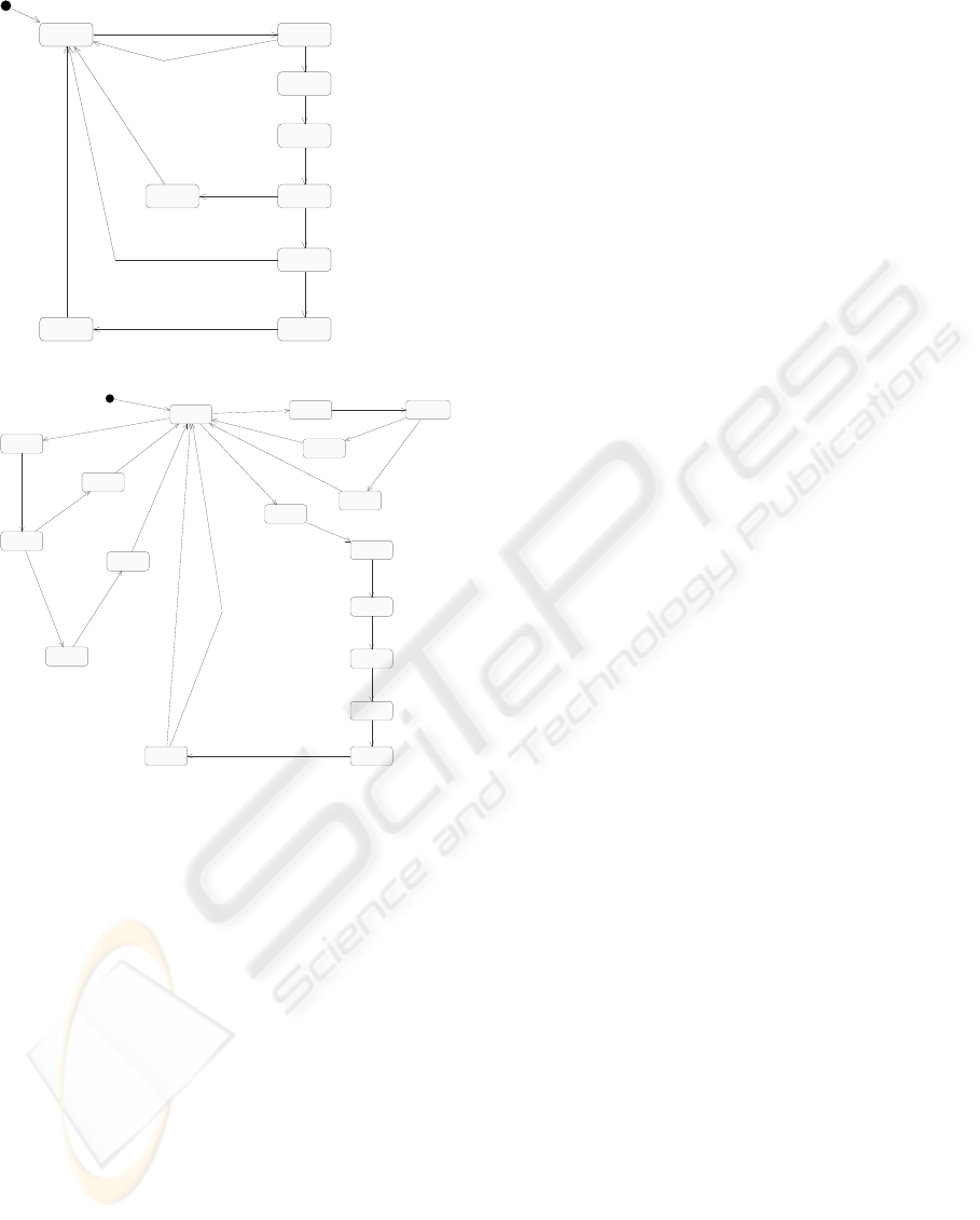
idle search
GetMerchantAcc
chargeAcc
findingAccaccNotFou
nd
accFound
chargedFro
mCust
validCharge
GetCustomerAccBalance
AccNotFind
AccFind
DepositToMerchant
SucceedAtCharge
wait
Charge
Charge
FailedAtMerchantAcc
SucceedAtMerchantAcc
FailedAtCharge
WithdrawFromCustom er
FailedAtCharge
(a) Statechart Diagram for Bank
idle
getProduct
waitProduct
GetProductInfo[ true && true
&& TCvar1 <= 2 ]
browseFail
ed
browseSuc
ceed
ProductNotFind[ true && true &&
true ] / true && TCvar2=0
AddressError[ true &&
true && TCvar2<=2 ]
ProductInfo[ true && true
&& true ] / true &&
TCvar3=0
Page[ true && true
&& TCvar3<=2 ]
startNegoti
ation
waitOthers
quantity
minPrice
riskFactor
AddStatistic[ true && true && true
] / sl’ = insert(s, sl)&& TCvar4 = 0
TotalQuantity[ true && true
&& TCvar4>=3 & TCvar4<=6
] / tq’ = totalQuantity(sl)
GetMinPrice / minprice =
getMinPrice(mid, pid, tq, rul)
GetRiskBalance / rf’ =
getRiskBalance(q/tq, ril)
acceptable
Price
CalculateAcceptablePrice / ap’ =
minprice * rf
negoResult
DeleteStatistic / sl’ = delete(s, sl)
BrowseAdd[ true &&
true && true ] / true &&
TCvar1=0
Item[ true && true && true ] / s’ =
create(uid, mid, pid, q, n) & uid1’ =
uid & mid1’=mid & pid1’ = pid & q1’ =
q & n1’ = n && TCvar5=0 & TCvar6 = 0
startInvoice
Purchase
askMercha
nt
succeed
failure
GenerateInvoice
InvoiceFailed[ true && true
&& TCvar8 <= 2 ]
Unsuccessful[ true &&
true && true ] / true
&& TCvar8=0
Successful[ true && true &&
true ] / true && TCvar7 = 0
commissio
n
AddCommission / cl’ =
insert(create(mid, invid,
amount), cl)
ReceiveInvoice[
true && true &&
TCvar7<=2 ]
Confirmed[ ap <= n1
&& true && TCvar5
>= 5 & TCvar5 <= 8
]
NotConfirmed[ ap
> n1 && true &&
TCvar6 >= 5 &
TCvar6 <= 8 ]
(b) Statechart Diagram for EBroker
Figure 3: Behavior Descriptions - 2
ceives back the reply SucceedMerchantAcc, and then
responds through the message Charge. At the end
of this sequence of message exchanges, they reach
the states startCharge and chargeAcc. The Merchant
agent waits in state startCharge until the Bank agent
completes a sequence of internal computations and
sends the message SucceedAtCharge to it. Upon re-
ceiving this message, the Bank agent goes to idle
state, the Merchant agent goes to succeed state. Af-
ter completing the internal computation to record the
invoice, the Merchant agent communicates to EBro-
ker through the message Successful and their states to
idle, and succeed. At this instance, the agents Bank
and Merchant are in their idle states, the agent EBro-
ker is in state succeed, and the agent User is in state
waitinvoice. The agent EBroker records the commis-
sion earned in this transaction within 2 time units of
receiving the message ReceiveInvoice and sends the
invoice to the User. Having sent the invoice, the
agent EBroker goes to its idle state. The agent User
executes the internal message Exit and goes into its
idle state.
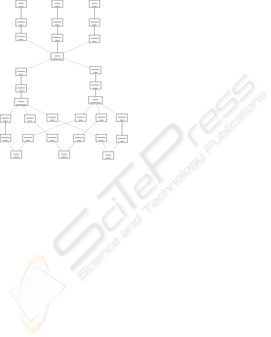
Figure 4 shows an E-commerce system configured
with three users, one E-broker, two merchants and
three banks. Each instance of User type models a
user with one port of type @A to communicate with
an agent of EBroker type. The E-broker agent in the
subsystem is an instance of EBroker agent type hav-
ing three ports of type @U, one port for each user; the
two ports of type @M are for communication with
the merchants in the system. Each merchant agent
in the system is an instance of Merchant agent type
with a port of type @G for communicating with the
broker agent, and three ports of type @B to commu-
nicate with the banks in the system. The agents are
linked through connectors at their respective compat-
ible ports for communication. For instance, the port
@A1 of user U 1 is linked to the port @U1 of the E-
broker E1. That link is not shared by any other agent.
Consequently, the architecture specification ensures
trust in communications.
The following section introduces a rigorous
methodology for predicting the reliability of E-
Commerce applications using Markov models con-
structed from a formal model of the E-Commerce ap-
plication.
3 MARKOV MODELS
Markov models are one of the most powerful tools
available to engineers and scientists for analyzing
complex systems. The basic concepts are explained
below.
3.1 Markov Models: Basic Concepts
Analysis of Markov models yield results for both the
time-dependent evolution of the system and the steady
state properties of the system. The Markov property
states that given the current state of the system, the
future evolution of the system is independent of its
history.
The Markov model of an E-Commerce component
may be represented by a state diagram. The states
represent the stages in the E-Commerce component
that are observable to the users, and the transitions be-
tween states have assigned probabilities. An algebraic
representation of a Markov model is a matrix, called
transition matrix, in which the rows and columns cor-
respond to the states, and the entry p
ij
in the i-th row,
j-th column is the transition probability for being in
state j at the stage following state i. We use tran-
sition matrix representation in reliability calculation
algorithms.
RELIABILITY ASSESSMENT OF E-COMMERCE APPLICATIONS
33
U1 :
User
U2 :
User
U3 :
User
@A1 :
@A
@A2 :
@A
@A3 :
@A
@U1 :
@U
@U2 :
@U
@U3 :
@U
E1 :
EBroker
@G1 :
@G
@G2 :
@G
M1 :
Merchant
M2 :
Merchant
@B1 :
@B
@B2 :
@B
@B3 :
@B
B1 :
Bank
B2 :
Bank
B3 :
Bank
@M1 :
@M
@M2 :
@M
@M3 :
@M
@B4 :
@B
@B5 :
@B
@B6 :
@B
@M4 :
@M
@M5 :
@M
@M6 :
@M
@C1 :
@C
@C2 :
@C
Figure 4: Subsystem Architecture
3.2 Discussion
Initial transition probabilities, obtained from various
sources including log files and other subjective opin-
ions of experts can not be used for predicting the re-
liability of the system. We contend that the reliabil-
ity should be calculated from the steady state of the
Markov system. A steady state or equilibrium state is
one in which the probability of being in a state before
and after transitions is the same as time progresses.
Computing the steady state vector for the transition
matrix of a large system is hard. However, as in our
approach, when the system is modularly constructed
it seems possible to partition the system into smaller
components, which might reduce the complexity of
computing steady state vectors.
3.3 Algorithm
We construct the Markov model of a E-Commerce
system in three steps. In the first step we construct
the Markov models for E-Commerce objects. In the
second step we construct the Markov models for every
pair of interacting objects in the system configuration
specification. Finally in the third step we construct
the Markov model for the fully configured system.
3.3.1 Step 1: Markov Models for Objects
We associate with each E-Commerce object in the
architecture another finite state machine, called its
Markov model. The states in the Markov model of
an object are the states of the object in its state ma-
chine description. A transition between two states in
the Markov model is defined only if there exists at
least one transition between those states in its state
machine. In the absence of statistical information
gathered by experts on the usage and failure, we will
assume that all the external events have equal proba-
bility in each state. For the transition from state i to
state j in the Markov model, a fixed probability p
ij
of
it going into state j at the next time step is calculated
as follows:
1. The initial probabilities for all the transitions in the
state machine of the reactive object are calculated.
The algorithm for calculating such probabilities for
a state is based on the following assumptions: 1)
all external events that can happen at the state have
the same probability; 2) all internal events that can
happen at the state have the same probability, and
(3) these are in general different.
2. In case there is more than one transition
{l
1
, . . . , l
n
} of the same type (shared/internal) from
state
i
to state
j
, then the above mentioned transi-
tions are substituted by one whose probability is
P = 1 − (1 − P{l
1
}) × . . . (1 − P {l
n
})
3. The probabilities of all the transitions for a state
have to sum to 1.
3.3.2 Step 2: Markov Model for Object Pairs
The interaction between two objects is due to shared
events. We compute the state machine for an interact-
ing pair of objects and compute the Markov model
with transition probabilities from the transitions at
each state of the product machine.
Algorithm for Transition Matrix for the
Synchronous Product Machine
Let E
1
and E
2
be the sets of internal events in the
statecharts P and Q of interacting objects, and F de-
note the set of shared events. Let M
1
and M
2
be the
transition matrices for P and Q. Let R be the syn-
chronized product machine of P and Q. Algorithm
SPM computes the transition matrix M of R by first
computing the synchronous product machine R, and
next determining the transition probabilities for tran-
sitions in each state of R. If all the transitions in a
state are labeled by internal events or if all of them
are labeled by shared events the probabilities are ob-
tained by normalizing the probabilities in their respec-
tive machines. However, if both internal events and
ICETE 2004 - SECURITY AND RELIABILITY IN INFORMATION SYSTEMS AND NETWORKS
34

shared events occur at the state, the probabilities for
the shared events are calculated first, and the remain-
ing measure is distributed to transitions labeled by in-
ternal events.
Algorithm SPM
Step 1. p = 1; // row sum
Step 2. x
1
= {e| e is a shared event occurring at
state i (P) and at state j (Q) }
x
2
= {e| e is an internal event occurring at state i
(P )} ∪ {e| e is an internal event occurring at state
j (Q) }
Step 3. If x
1
6= ∅ // calculate probabilities for tran-
sitions due to shared events
then NF = 0 (Normalization Factor); set
1
= ∅;
Step 3.1 For each event e ∈ x
1
find the (set of)
states i
0
(P ) and j
0
(Q) such that i
e
→ i
0
, j
e
→ j
0
Step 3.2 y = y ∪ {i
0
, j
0
}, if {i
0
, j
0
} /∈ y
Step 3.3 NF = N F + M
1
[i, i
0
] × M
2
[j, j
0
]
Step 3.4 M[(i, i
0
), (j, j
0
)] = M
1
[i, i
0
]×M
2
[j, j
0
]
Step 3.5 set
1
= set
1
∪ (j, j
0
)
Step 4. If x
2
6= ∅ // calculate probabilities for tran-
sitions due to internal events
then NF
0
= 0 (Normalization Factor); set
2
= ∅;
Step 4.1 For each event e ∈ x
2
, if e ∈ M
1
then
find the state i
0
(M
1
) such that i
e
→ i
0
;
y = y ∪ {i
0
,j} if {i
0
,j} /∈ y;
M[(i, j)(i
0
, j)] = M
1
[i, i
0
]; N F
0
= NF
0
+
M[(i, j)(i
0
, j)];
set
2
= set
2
∪ (i, i
0
)
else
find the state j
0
(M
2
) such that j
e
→ j
0
;
y = y ∪ {i, j
0
} if {i, j
0
} /∈ y;
M[(i, j)(i, j
0
)] = M
2
[j, j
0
]; NF
0
= NF
0
+
M[(i, j)(i, j
0
)];
set
2
= set
2
∪ (j, j
0
)
Step 5. If x
1
= ∅ ∧ x
2
= ∅, the (i, j) row is deleted
from M
Step 6.If x
1
= ∅ ∧ x
2
6= ∅
For each (i
0
, j
0
) ∈ set
2
do
M[(i, j), (i
0
, j
0
)] =
M[(i, j), (i
0
, j
0
)]
NF
0
Step 7. If x
1
6= ∅ ∧ x
2
= ∅
For each (i
0
, j
0
) ∈ set
1
do
M[(i, j), (i
0
, j
0
)] =
M[(i, j), (i
0
, j
0
)]
NF
Step 8. If x
1
6= ∅ ∧ x
2
6= ∅ do
For each (i
0
, j
0
) ∈ set
2
do
M[(i, j), (i
0
, j
0
)] =
(1 − NF ) × M[(i, j), (i
0
, j
0
)]
NF
0
Step 9. Fill in the matrix M with 0 where there are
no entries.
3.3.3 Step 3: Markov Model for a System
A system configuration, when partitioned into slices
based on synchronization criteria, produces two types
of subsystem components: (1) linear configuration,
and (2) non-linear configuration. As an illustration, a
simple system in which one user is interacting with
a browser to access information, as shown in Fig-
ure 5(a) is linear, whereas the system in which users
join the system at different times, as shown in Fig-
ure 5(b) is non-linear.
Case 1: Linear System
In a linear system, objects synchronize in the past.
If o
1
, . . . , o
n
are objects in the linear system and
M
1
, . . . , M
n
are respectively their transition matri-
ces, then the transition matrix M of the linear system
is computed as follows:
1. Compute M = M
1
⊗M
2
(Apply Algorithm SPM)
2. for j = 3 to n compute M = M ⊗ M
j
(Apply
Algorithm)
Case 2: Non-linear System
In a non-linear system, as in Figure 5(b), several ob-
jects interact with an object. These interactions may
be initiated at different times. The synchronous prod-
uct machine dynamically changes as and when ob-
jects join or leave the system, and hence the transition
probability matrices also change, and should be re-
computed. We explain the computation procedure for
Figure 5(b). For simplicity of discussion we assume
that users join the system one at a time, but don’t leave
the system. Let 0, k
1
, k
2
, . . . , k
n−1
be the intervals of
successive arrivals of users. That is, for j > 1 the
j-th user joins the system k
j−1
(> 0) time units after
j − 1-st user joined the system. Let M
1
be the transi-
tion matrix of the Markov model for the linear system
computed at time step k. The transition matrix for
M
(n)
, n ≥ 2, users interacting with one browser and
one server object is calculated as follows:
RELIABILITY ASSESSMENT OF E-COMMERCE APPLICATIONS
35

User Server
Browser
Ini
synchronize
synchronize
(a) Linear Architecture
User User UserUser
1 2 3 n
Server
Browser
(b) Non-Linear Architecture
Figure 5: Linear and Non-Linear Models
M
(2)
= M
k
1
1
L
M
1
M
(3)
= [M
(2)
]
k
2
L
M
1
.
.
.
M
(j)
= [M
(j−1)
]
k
j−1
L
M
1
, 2 ≤ j ≤ n
.
.
.
In the above calculation, the symbol
L
denotes the
direct product operator for matrices. The justification
for direct product computation is based on the obser-
vations:
• the event received by the system from a new User
object can come only when the system is in any one
of its states in which it can be accepted,
• the incoming event is not time-constrained with re-
spect to the Markov model of the system. that
is M
1
for the new interaction is independent of
[M
(j−1)
]
k
j−1
, and
• when a new object joins the system the size of the
new Markov matrix increases m-fold, where m is
the size of the Markov matrix of the new object.
For the non-linear system in Figure 5(b), assume that
four users join the system,one at a time, at times 0,
2, 4, 5. So, k
1
= 2; k
2
= 2; k
3
= 1. The transition
matrix of the system at different time points are shown
below:
At time 0 or 1: (1 user): M
1
At time 2: (2 users): M
(2)
= M
2
1
L
M
1
At time 4: (3 users): M
(3)
= [M
(2)
]
2
L
M
1
At time 5: (4 users): M
(4)
= [M
(3)
]
L
M
1
Let us consider the general case when r > 1 users si-
multaneously join the system, say when there are j−1
users in the system. It is easy to see that the transition
matrix for the new configuration with r + j − 1 users
is M
(r+j−1)
= [M
(j−1)
]
k
j−1
L
M
(r)
1
, where M
(r)
1
is the direct product M
1
L
M
1
L
. . . M
1
, taken r
times. When r users leave the system, the transition
matrix is computed as follows: Let there be j(≥ 2)
users in the system when r(1 < r ≤ j) users leave.
If r = j, then the transition matrix is not defined. If
r < j, there are j − r users left in the system. If d
is the interval of time that elapsed between the latest
time when there were j − r users in the system and
the current instant, then the new transition probability
matrix is [M
(j−r)
]
d
. The rationale is that the transi-
tion probability matrix M
(j−r)
for j − r users have
evolved over d time steps.
For the E-Commerce system shown in Figure 4
the Markov matrix can be computed using the above
method. The details are left to the reader.
4 RELIABILITY MEASURES
We define the reliability prediction for a system con-
figuration composed from k objects as the level of cer-
tainty quantified by the source excess − entropy:
Reliability(Subsystem) =
k
X
i=1
H
i
− H
where H = −
P
i
v
i
P
j
p
ij
log p
ij
is a level of
uncertainty of the Markov system corresponding to a
subsystem; v
i
is a steady state distribution vector for
the corresponding Markov system and the p
ij
values
are the transition probabilities. H
i
is a level of un-
certainty in a Markov system corresponding to a reac-
tive object. For a transition matrix P the steady state
distribution vector v satisfies the property vP = v.
The level of uncertainty H is related exponentially to
the number of paths that are ”statistically typical” of
the Markov system. Thus, higher entropy value im-
plies that more sequences must be generated in order
to accurately describe the asymptotic behavior of the
Markov system.
The reliability prediction for a system is defined as
the least reliability measure value among its m sub-
systems:
Reliability(System) =
min{Reliability(Subsystem
i
)}
m
i
We chose the minimum value due to the safety-critical
character of the real-time reactive systems. Higher
value of reliability measure implies less uncertainty
present in the model, and thus higher level of software
reliability.
The Markov model of a configured system changes
when the system undergoes change. The calcula-
tion of the Markov matrix for the reconfigured sys-
tem would allow to compare the systems based on re-
liability prediction. If the system configuration C
j−1
ICETE 2004 - SECURITY AND RELIABILITY IN INFORMATION SYSTEMS AND NETWORKS
36

changes to the configuration C
j
, we need to calculate
the reliability of the configuration C
j
and compare it
with the reliability of the configuration C
j−1
:
Reliability(C
j−1
) = min{Reliability(S
i
)}
m
i
,
where S
i
is a subsystem of C
j−1
, and
Reliability(C
j
) = min{Reliability(S
0
i
)}
m
i
,
where S
0
i
is a subsystem of C
j
. If Reliability(C
j
) ≥
Reliability(C
j−1
), then the uncertainty present in
the reconfigured system is less than the uncer-
tainty that existed in the current system. The
reliability measurement will allow the reconfig-
ured system to be deployed. However, if
Reliability(C
j
) < Reliability(C
j−1
), then there is
more uncertainty present in the reconfiguration. This
would suggest to determine the subsystem(s) of C
j
that are responsible for lowering the overall reliabil-
ity.
5 CONCLUSIONS AND
RESEARCH DIRECTIONS
The goal of this paper is to show that a rigorous ap-
proach to reliability prediction of E-Commerce sys-
tems is possible, when we construct a formal model
of it. The E-Commerce model introduced in this pa-
per is simple, yet a realistic model which is complex
enough to serve as a test bed for experimentation. In
a practical setting, the number of E-Commerce com-
ponents and their interactions will be much larger.
There are also other factors such as resource con-
straints, load factor, and communication complexity.
From a reliability point of view, we require a good
formal model which takes these factors into account.
In the formal model proposed in this paper the load
factor and communication delays can be brought in
as synchronization constraints, and resources can be
modeled within each class and timing constraints may
be imposed on database transactions. Calculation of
transition probabilities for large evolving configura-
tions involves multiplying fairly large matrices. The
density of the transition probability matrix of a sys-
tem depends on the number of transitions in the prod-
uct matrix, which due to synchronization constraints,
might be sparse. The sparsity of the matrix and the
availability of very fast powering and multiplication
algorithms for matrices may be used to speed up reli-
ability calculation for changing configurations.
Our research is based on the premise that E-
Commerce systems should be analyzed for several
improperties before deployed for public use. Secu-
rity and reliability are two important properties. Re-
liability promotes trust and security preserves trust.
We have a full implementation of the reliability cal-
culation based on the methods discussed in this pa-
per. One of our ongoing efforts is centered on for-
malizing security policies and integrating them with a
component-based implementation of our model.
REFERENCES
In IEEE Standard Glossary of Software Engineering Termi-
nology. IEEE 610.12.1990.
In FIPA Communicative Acts Library. FIPA Specification
Repository (2001). Foundation for Intelligent Physical
Agents, G.
Alagar, V., Holliday, J., Thiagarajan, P., and Zhou, B.
(2002). Agent types and their formal descriptions. In
Technical Report, Department of Computer Engineer-
ing, Santa Clara University, Santa Clara, California,
U.S.A.
Franklin, S. and Graesser, A. (1996). Is it an agent or
a program?: A taxonomy for autonomous agents.
In Proceedings of the Third International Workshop
on Agent Theories, Architectures, and Languages.
Springer-Verlag.
Kallepalli, C. and Tian, J. (Nov. 2001). Measuring and
modeling usage and reliability for statistical web test-
ing. In IEEE Transactions on Software Engineering,
(Vol.27, No.11), pp.1023–1036. IEEE.
Ormandjieva, O. (2002). Deriving new measurements for
real-time reactive systems. In Ph.D. thesis, Concordia
University, Montreal, Canada.
Papazoglou, M. P. (April 2000). Agent-oriented technology
in support of e-business. In Communications of the
ACM, Vol.44. No.4.
RELIABILITY ASSESSMENT OF E-COMMERCE APPLICATIONS
37
